LTB and steel columns: effective length, resistance and interaction
This lecture completes B2/B3 LTB, uses an overhanging beam to explain load patterns, then introduces columns. Keep section resistance and overall member stability as two levels. , , and describe different instability problems throughout the lecturer's method.
Abbreviations: DL—Dead Load; LL—Live Load; ULS—Ultimate Limit State; SLS—Serviceability Limit State; UDL—Uniformly Distributed Load; LTB—Lateral-torsional Buckling; UB—Universal Beam; UC—Universal Column.
Key Points
- Passing does not prevent LTB of the whole beam. Without intermediate restraint, calculate separately.
- LTB sequence: →→→read , interpolating if required→.
- For overhanging beams, separate load patterns and draw shear and moment diagrams for each.
- Columns need section checks using and member checks using . Calculate both axes and use the smaller .
- Eccentric beam reactions create column moments, distributed according to upper/lower segment stiffness.
Key Formulas
Exam Question Types
- LTB check for a beam without intermediate restraint. → Unrestrained B2: a strong section can still buckle (Unrestrained Beam)
- LTB with midspan restraint and table interpolation. → B3 with midspan restraint: complete the LTB procedure (Restrained Segments)
- Pure-compression column resistance. → Pure-compression UC column: from two-axis lookup to capacity (Axial Compression)
- Eccentric moments in a simple-construction column. → Simple-construction column: how beam reactions produce moments (Beam Reactions into Columns)
Design flows for these question types
- Breaks and waiting periods have been omitted.
- The overhanging beam has two load patterns. This page completes segment AB; the lecturer does not finish BC.
B2: lack of intermediate restraint reduces resistance (Unrestrained B2)
What this unit is for: The section of B2 is strong enough in bending, but nothing holds its compression flange along the whole span; this unit finds its capacity against lateral-torsional buckling.
Picture it this way: Work the two sides separately. Capacity side: from the unheld length and get the slenderness, convert it to , read off , which is far smaller than , and obtain . Demand side: take from the shape of the moment diagram and multiply the largest moment. Compare only when both are in kNm.
Prerequisites: Why a beam moves sideways and twists (Lateral-torsional Buckling) · Instability can precede material crushing (Buckling) · Read an I-section and its section table (Section Properties)
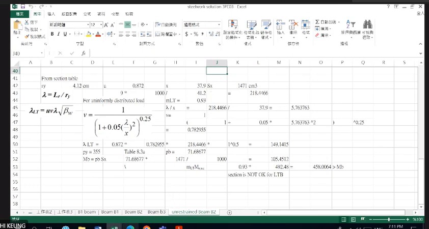
B2 passed cross-sectional bending in the previous lecture, but here the 9 m length has no effective intermediate lateral restraint. The compression flange can move sideways and twist the section. Calculate separately; is not the stability resistance.
Convert 9 m to 9000 mm and divide by . The resulting 218.45 is ordinary slenderness . Apply , and the other parameters to obtain before reading . This resembles using column to read , but the tables and factors differ.
comes from moment distribution and acts on demand; comes from the stability curve and acts on resistance. The example keeps these paths separate until the final comparison in kNm.
Complete worked examples in this unit: Unrestrained B2: a strong section can still buckle (Unrestrained Beam)
B2: inadequate without intermediate lateral restraint
B2 uses an unrestrained length of 9 m and , giving and then .
The lookup gives and . Demand greatly exceeds resistance.
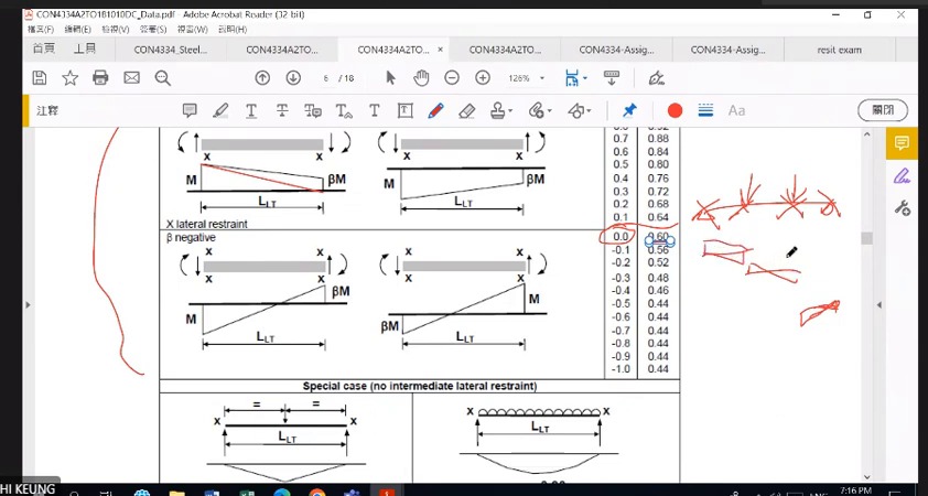
Equivalent uniform moment factor
represents the moment distribution within the unrestrained segment. Select it using end-moment signs and diagram shape.
The displayed case gives . Other loading forms or intermediate loads require their corresponding table cases; 0.60 is not universal.
Unrestrained B2: a strong section can still buckle (Unrestrained Beam)
Beam B2 is a 457×191×67 UB. Nothing holds it sideways along its 9000 mm length. The largest moment is 492.48 kNm. Decide whether the beam will move sideways and twist (lateral-torsional buckling).
Solution Route: Confirm no intermediate restraint→convert to with course parameters→read →calculate →adjust demand.
B3: midspan restraint and table interpolation (Restraint and Interpolation)
What this unit is for: B3 has its compression flange held at mid-span, which halves the length that can buckle; this unit uses the shorter length in the tables and interpolates between two rows.
Picture it this way: The compression flange acts like a long pole being squeezed. Hold it at the middle and it becomes two shorter poles that are much harder to bow out. Interpolation is like reading a ruler between two marks: the answer always lies between the two marks, nearer to the closer one.
Prerequisites: Why a beam moves sideways and twists (Lateral-torsional Buckling) · Instability can precede material crushing (Buckling)
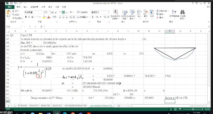
B3 is 6 m long, but midspan lateral restraint reduces the analysis segment to 3 m. Circle adjacent restraint points before entering . The presence of “6 m” in the question does not automatically mean using 6000.
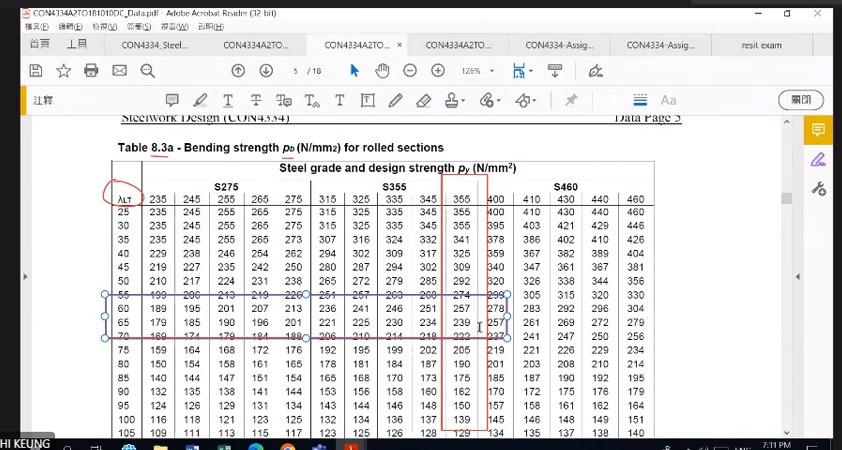
Read tables in two directions: select the column, then locate rows. Interpolate linearly only between adjacent rows and check that the result lies between their values. This catches a reversed interpolation sign immediately.
Here 60.86 is close to 60, so should be closer to 257 than to 239. Calculate the interpolation fraction, then ; retain intermediate precision and round appropriately at the end.
Complete worked examples in this unit: B3 with midspan restraint: complete the LTB procedure (Restrained Segments)
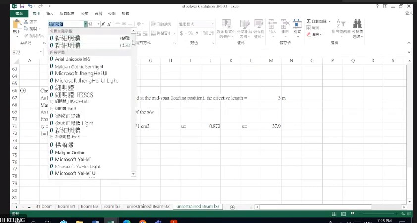
How to read this image: Read , then , , and . Do not retain B2's 9 m.
Lookup and interpolation: from to
Select the column first, then the row. Thickness affects ; S355 does not mean every section uses 355.
The course interpolates linearly between rows. B3 has and .
B3: a midspan restraint shortens effective length
The beam spans , but midspan restraint gives for this segment. Parameters are , , and .
From and , obtain and . With moment-diagram , take .
- Confirm lateral-restraint positions first. Do not take the whole 6 m span as this segment's .
- Use for the Class 1/2 case here; calculate before the lookup.
- Resistance is ; multiply demand separately by . The comparison passes LTB for this segment.
B3 with midspan restraint: complete the LTB procedure (Restrained Segments)
Beam B3 is a 457×191×67 UB spanning 6 m. It is held sideways at both ends and at mid-span, so each unrestrained length is 3000 mm. The largest moment is 333.144 kNm. Decide whether this length fails by lateral-torsional buckling.
Solution Route: →→→→→; separately derive from the moment diagram, then compare demand and resistance.
Overhanging beam Q5: separate load patterns before internal actions (Load Patterns)
What this unit is for: One end of the beam sticks out past its support, and load on that overhang changes the moment in the main span; this unit separates the load arrangements, then checks the length between the supports.
Picture it this way: When someone sits on one end of a see-saw, the other end lifts. Load on the overhang levers the main span upwards in the same way and reduces the moment in the middle of the main span. The worst arrangement for the main span is therefore full load on the main span with less load on the overhang.
Prerequisites: Turn the physical structure into a calculation model (Free-body Diagram) · Internal shear force and bending moment in a beam (Shear Force and Bending Moment) · Why a beam moves sideways and twists (Lateral-torsional Buckling)
Overhang loading creates negative moment at the right support and changes the left reaction . Changing only the overhang load therefore also changes main-span moment. Treating the two spans as unrelated simply supported beams loses equilibrium.
The lecturer uses different loading patterns to check different segments. Case 1 has maximum main-span loading and lower overhang loading, giving about 393.3 kNm. Another diagram increases overhang loading and gives about 369.9 kNm and support moment −99 kNm. These are different patterns, not before-and-after corrections.
The worked example fills in support equilibrium, the zero-shear location and maximum moment, then follows the course quarter-point moments to . Each number can be traced from the free-body diagram rather than memorised as a special overhang answer.
Complete worked examples in this unit: Overhanging beam Q5: separate load patterns and check AB (Overhanging Beam)
Overhanging beam Q5: establish the load model
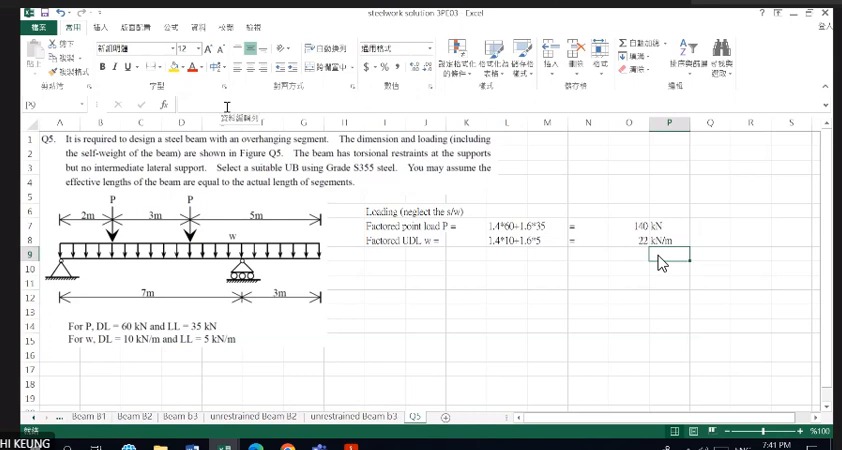
Point loads lie 2 m and 5 m from the left end. Supports are at 0 m and 7 m; the beam extends to 10 m.
Each point load has DL=60 and LL=35 kN, giving design value 140 kN. UDL components DL=10 and LL=5 kN/m give 22 kN/m. Self-weight is neglected as specified.
Draw shear and moment diagrams before selecting a section
The overhang creates negative moment at the right support, so maximum positive moment need not occur at geometric midspan. Find reactions by equilibrium, then construct shear and moment piecewise.
Trial flange thickness gives on screen. Do not automatically use 355 merely because the steel is S355.
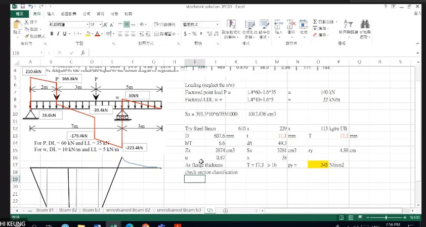
How to read this image: Read BC total load 30 kN and , then note requires .
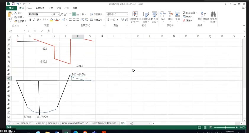
How to read this image: Here and support negative moment is 99. Record these separately from Case 1's 393.3.
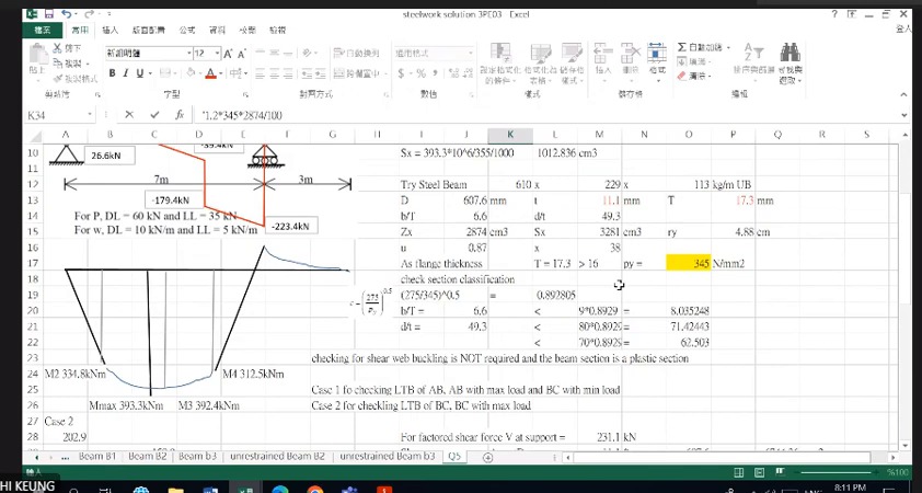
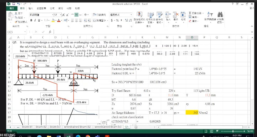
How to read this image: Read the Case 1/Case 2 descriptions, then take , and from the same diagram for .
LTB check for segment AB between supports
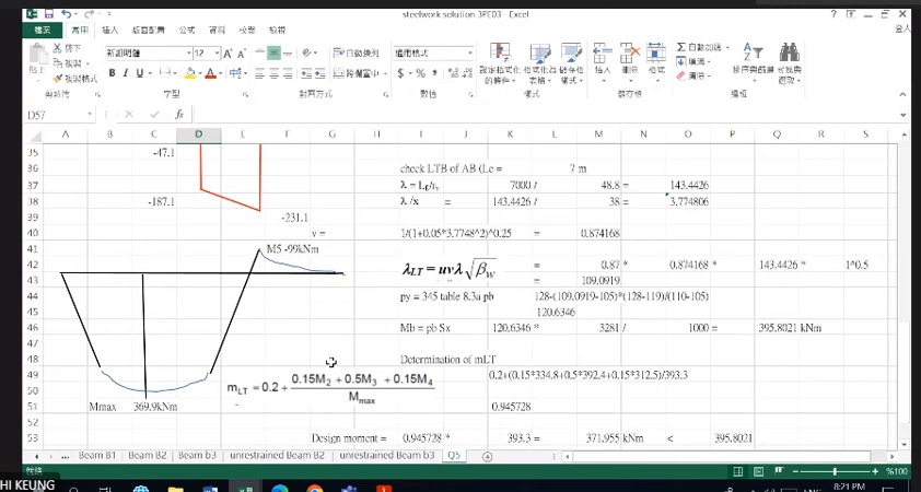
Here and . With and , .
The screen gives and , hence . Segment moments give and demand about 371.96 kNm, below resistance.
Overhanging beam Q5: separate load patterns and check AB (Overhanging Beam)
A beam rests on supports and , 7 m apart, and sticks out 3 m beyond to . It carries two point loads and a uniform load. Find the reactions and the largest moment, choose a section, then check span AB for lateral-torsional buckling.
Solution Route: Factored loads→specified pattern→moment equilibrium/reactions →piecewise shear/moment→section selection→AB LTB.
Introducing columns: effective length and two checking levels (Column Design Levels)
What this unit is for: A column can be crushed at one cross-section, or the whole column can bow sideways; this unit tells the two checks apart and explains what effective length means.
Picture it this way: A short stick of chalk is crushed when squeezed; a long strand of dry spaghetti bows sideways instead. These are different failures. Grip both ends of the spaghetti so they cannot rotate and it is harder to bow. Effective length turns that help from the ends into a single length.
Prerequisites: Instability can precede material crushing (Buckling) · Combined axial force and bending (Interaction Checks) · Will the plate buckle before its material strength is fully mobilised? (Section Classification)
A column can exhaust section compression strength or buckle over its length. Section checks use ; member checks use buckling-reduced . Dividing the same axial force by these different capacities distinguishes the two questions.
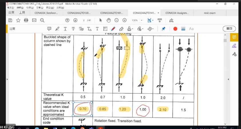
Effective length incorporates end rotation and sway restraint into an equivalent length. Tables list ideal and approximate practical values. The lecturer warns against mixing assumptions from different rows in one problem.
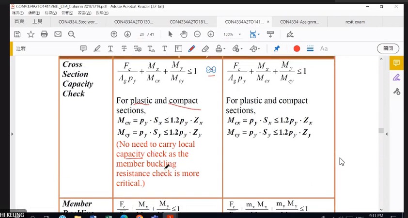
For biaxial bending, calculate section capacities separately about and . For Class 1/2, each uses the smaller of and 1.2pyZ; the weak-axis cap can govern. Member expressions use their own course denominators and factors, not a copied section-check row.
Column end restraints and effective length
Effective length represents the column's buckling shape as an equivalent length. Both rotational and translational restraints affect .
The ideal fixed–fixed theoretical value is , whereas the approximate practical recommendation is 0.70. For other supports too, stay within the same table row of assumptions.
Axial compression plus biaxial bending: section check
is the design axial compression at the same critical section; and are its two bending moments . is gross area.
This checks section strength without column length or overall buckling reduction. Do not apply the simplified expression directly to Class 4 sections.
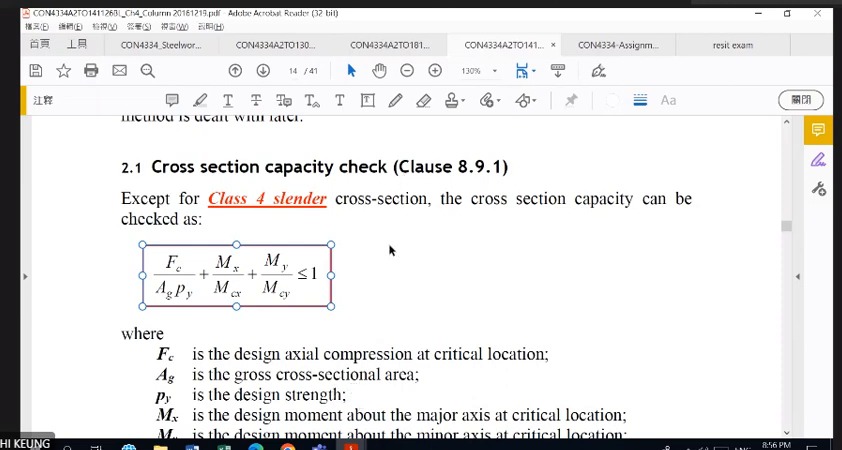
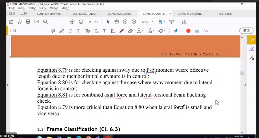
How to read this image: Locate and first, then identify which demand term each of , and multiplies.
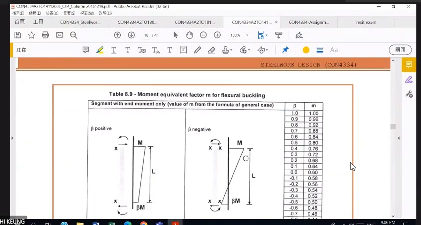
How to read this image: Use the diagram's convention to select the correct row. Negative- cases cannot all be handled with one straight-line formula.
Section and member checks cannot replace each other
For Class 1/2, take the smaller of plastic resistance and the 1.2-times-elastic cap.
Member-buckling checks instead use slenderness -reduced and the relevant moment factors, or elastic capacities. Do not transfer denominators indiscriminately between expressions.
Pure compression: two-axis slenderness and governing curves (Axial Column)
What this unit is for: A column can bow in two directions, and the weaker direction decides how much compression it can take; this unit looks up each axis separately and takes the smaller value.
Picture it this way: Squeeze a flat ice-lolly stick from both ends and it always bows towards its thin side, never its wide side. A column has a weaker direction too. So each direction gets its own slenderness and its own compressive strength, and the smaller strength is the one used.
Prerequisites: Instability can precede material crushing (Buckling) · Read an I-section and its section table (Section Properties)
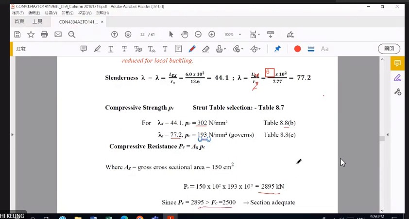
Different radii of gyration represent different material distributions for bending about the principal axes. Even with equal effective lengths , and differ. Calculate them in separate columns and select each buckling curve separately.
is not material yield strength . It is design compressive strength derived from member slenderness and the buckling curve. Select the governing axis value and multiply by area to obtain a force comparable with 2500 kN.
Weak-axis strength 193 N/mm² governs here, giving 2895 kN. The example also links to the later 4.5 m case using the same section, showing how shorter effective length changes and resistance.
Complete worked examples in this unit: Pure-compression UC column: from two-axis lookup to capacity (Axial Compression)
Pure axial compression example: list the conditions first
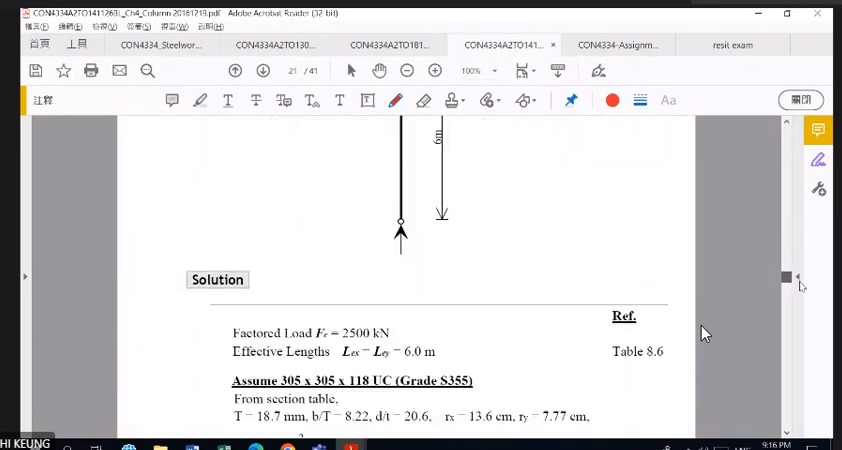
Trial section 305×305×118 UC, S355, ; effective lengths are 6 m about both axes.
The table gives , , and . Make length units consistent before calculating.
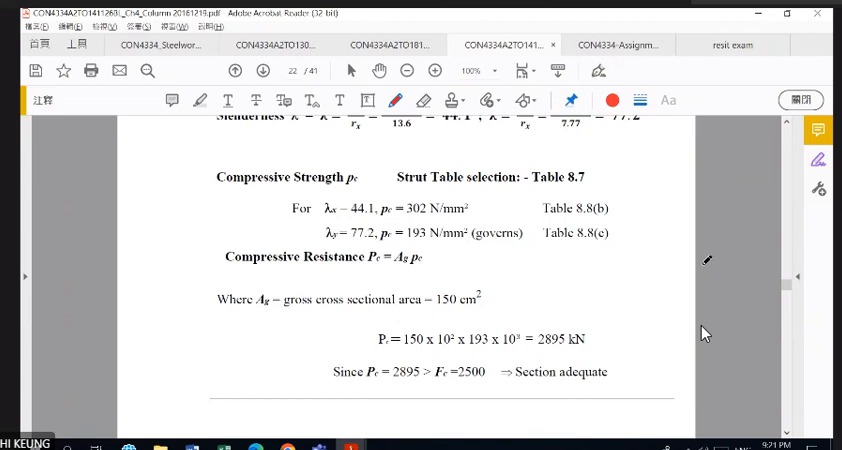
How to read this image: Identify -axis 302 and -axis 193, choose the smaller, then use 150 cm² to obtain 2895 kN.
Read both axes and take the lower compressive strength
After selecting the appropriate curve for each section/axis combination, -axis is smaller and governs.
exceeds 2500 kN. This pure-compression example passes.
Pure-compression UC column: from two-axis lookup to capacity (Axial Compression)
S355 steel column is pinned at both ends, with an effective length of 6 m, and carries a compression force of 2500 kN. A 305×305×118 UC is tried. Decide whether the column can carry this force without buckling.
Solution Route: Consistent units→two-axis slenderness →axis-specific curves→compare →capacity versus demand.
Beam–column eccentricity and distribution between column segments (Simple Construction)
What this unit is for: A beam reaction lands on one side of the column, not on its centre, so the column is bent; this unit finds that moment and shares it between the column lengths above and below.
Picture it this way: Carry a heavy bag in one hand and your body is pulled to that side, because the weight is off your centre line. A beam resting on one side of a column bends it likewise, with the distance measured to the column centre. The column lengths above and below share this moment; the shorter, stiffer one takes more.
Prerequisites: How loads travel from the slab to the ground (Load Path) · Why the position of a force matters (Moment and Eccentricity) · Combined axial force and bending (Interaction Checks)
A beam-end reaction acting away from the column centre creates an eccentric moment. Measure from the connection to the column centre; do not use only the 100 mm beyond the face and omit half the column depth.
Distribute joint moment between the upper and lower column segments. For equal sections, the shorter segment has greater rotational stiffness and takes more. The 6 m and 3 m segments here do not split equally. Equal stiffness in the next lecture does justify a half-and-half split.
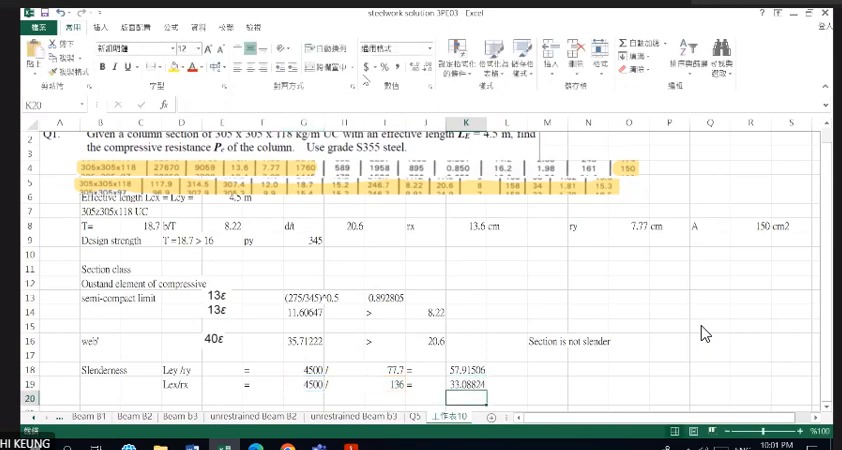
Finally, Q1 changes the pure-compression effective length to 4.5 m. Read again for this new condition; the same section designation does not justify copying the 6 m resistance.
Complete worked examples in this unit: Simple-construction column: how beam reactions produce moments (Beam Reactions into Columns)
Moment terms for a column in a simple multistorey structure
This particular simple-construction method takes moment factors as 1 and uses . It is conditional, not a method for every rigid-frame column.
The -axis candidates are 232.9 and 248.8 kNm; use 232.9. The -axis candidates are 108.3 and 85.6 kNm; use 85.6. The weak-axis 1.2pyZ cap can govern.
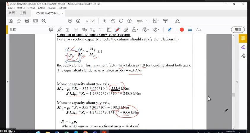
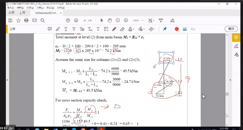
How to read this image: Calculate , then 362 kN producing 74.2 kNm. Distribute 49.5 and 24.7 according to the 6 m/3 m segments.
Q1: effective length changes to 4.5 m
The section is the same as the 6 m example, but falls to 4.5 m and weak-axis slenderness to approximately 57.9.
The lecturer completes this step on 31 October in Q2: weak-axis , giving with .
Simple-construction column: how beam reactions produce moments (Beam Reactions into Columns)
A main beam delivers reactions of 42 kN and 320 kN to the side of a 203×203×60 UC column, not at its centre, so the column bends. The column lengths above and below are 6000 and 3000 mm. Find the column moment and do the section check.
Solution Route: Eccentricity →joint moment→upper/lower distribution→amplified demand→section comparison.