Overhanging beam Q5: separate load patterns and check AB (Overhanging Beam)
Task: Find reactions and maximum positive moment from the complete free body, and understand different loading patterns for different unrestrained segments.
Go straight to Step 1 ↓Design flow for this type of question: Unrestrained beam (lateral-torsional buckling) →
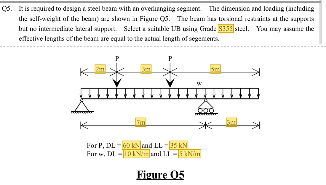
The question in short: A beam rests on supports and , 7 m apart, and sticks out 3 m beyond to . It carries two point loads and a uniform load. Find the reactions and the largest moment, choose a section, then check span AB for lateral-torsional buckling.
What differs from the previous example of this type: In the two earlier examples the moment was given. Here the loads must first be factored, the reactions found and the moment diagram drawn, and the overhang load is arranged in different patterns that give different moments.
| Given | Value and Unit |
|---|---|
| Geometry | Span AB 7 m, overhang BC 3 m; point loads 2 m and 5 m from |
| Loading | Each : dead 60 kN, imposed 35 kN; UDL: dead 10 kN/m, imposed 5 kN/m (self-weight included) |
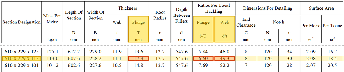
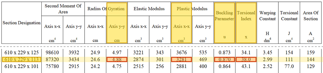
| Section | S355; trial 610×229×113 UB; ; ; ; ; , |
Yellow: values given in the question. The same values are marked where they are substituted in the steps below.
Orange box: values read directly from the Data File, the same values boxed orange in the lookup screenshots. A value interpolated between two table rows is a calculation, so it has no box.
Solution Route: Factored loads→specified pattern→moment equilibrium/reactions →piecewise shear/moment→section selection→AB LTB.
The beam takes the loads to supports and . Load on the overhang BC levers span AB upwards, so how much load BC carries changes the moments in AB.
- Design loads;
- Support reactions;
- Largest sagging moment in ABAbout 393.19 kNm (where )
- Hogging moment at−45 kNm
- Lateral-torsional buckling of ABDemand 371.96 kNmCapacity 395.8 kNmUtilisation 0.94
- Step 1 · Combine loads first
Why this step: Load factors increase the loads to leave a safety margin. Imposed load is harder to predict than dead load, so its factor is larger.
140 and 22 are this problem's maximum design values. Case 1 shows only total 30 kN on BC; reproduce that diagram without treating it as a universal load-combination rule.
- Step 2 · Case 1 equivalent actions
Why this step: Load on the overhang levers span AB upwards and reduces its sagging. So full load on AB with the least load on BC gives the largest sagging moment within AB.
Case 1: the full design UDL of 22 kN/m on AB; BC carries dead load only with a factor of 1.0, that is 10 kN/m × 3 m = 30 kN (the lecturer’s load case). These equivalent point loads are only for overall equilibrium; internal forces still follow the distributed loads.
New symbols in this step- , , , : Course LTB section/conversion parameters; dimensionless
Where the numbers come from: from Step 1.
- Step 3 · Take moments about
Why this step: The beam does not rotate, so the turning effects of all forces about must cancel. Taking moments about leaves out the unknown , so one equation gives .
Either rotation sign convention works if used consistently. BC loading to the right rotates about in the opposite sense to loading on the left.
Where the numbers come from: from Step 1; from Step 2; from Step 2.
- Step 4 · Vertical equilibrium
Why this step: The beam does not move up or down, so the two upward reactions must exactly carry all the downward loads. Once one reaction is known, the other follows.
Subtract from total load 464 kN to obtain . The drawing rounds to 210.6, causing small subsequent rounding differences.
Where the numbers come from: from Step 1; from Step 2; from Step 2; from Step 3.
- Step 5 · Find between the point loads
Why this step: Where the shear changes from positive to negative, the moment stops rising and starts to fall. That point is where the moment is largest and the beam is bent hardest.
For , one 140 kN load lies to the left. In a continuously loaded region, a moment maximum or minimum occurs where .
Where the numbers come from: from Step 3; from Step 1; from Step 1.
- Step 6 · Substitute into the segment moment expression
Why this step: This largest sagging moment puts the bottom of the beam in tension and the top in compression. It is the demand for choosing the section and the used later in the lateral-torsional buckling check of AB.
Take moments of the left-hand forces about the cut. With rounded reactions , the course diagram gives about 393.3 kNm.
New symbols in this step- , , , : Quarter-point and maximum moments from the same load case; kNm
- Step 7 · Check negative support moment
Why this step: The overhang acts like a diving board. Its load bends it down, so at the top of the beam is in tension and the bottom in compression, the opposite of mid-span.
BC UDL produces hogging moment at . Its presence does not mean is a fixed support.
Where the numbers come from: from Step 2.
- Step 8 · Keep the second load case distinct
Why this step: With full load on BC, the hogging moment at is largest. This is the worst case for the overhang and the support, but it also reduces the sagging moment in AB.
Another screen also applies maximum UDL22 kN/m to BC, giving moment −99 kNm and positive moment about 369.9 kNm. 393.3 and 369.9 belong to different patterns, not two answers to one expression.
Load path · Load, shear force and bending momentLoad on the overhang BC levers span AB upwards: the more load on BC, the larger the hogging moment at and the smaller the sagging moment in AB. So AB is checked with dead load only on BC (case 1), and BC and support with the maximum load on BC (case 2).
Case 1: , and are the quarter-point moments of AB from the class sheet, used to find . Case 2: the hogging moment at rises to −99 kNm and the largest sagging moment in AB falls to about 369.8 kNm (369.9 on the class sheet). - Step 9 · Reselect strength from thickness
Why this step: If the flange or web is too thin, it wrinkles locally in compression before the section reaches its full strength. Classification confirms they are stocky enough to use . Thicker steel also has a lower .
Trial gives course . Classification uses , and the corresponding limits.
New symbols in this step- , : Design yield and bending buckling strengths; N/mm²
Data file lookup · Data Page 1 · Design strength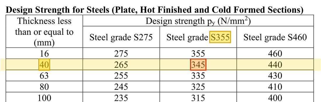
Flange thick: the row, S355 column gives . How the grade and thickness choose this row →Yellow: given parameter, row or columnOrange: value read from the table, boxed orange in the text too Data file lookup · Data Page 1 · Table 7.1 Limiting width-to-thickness ratios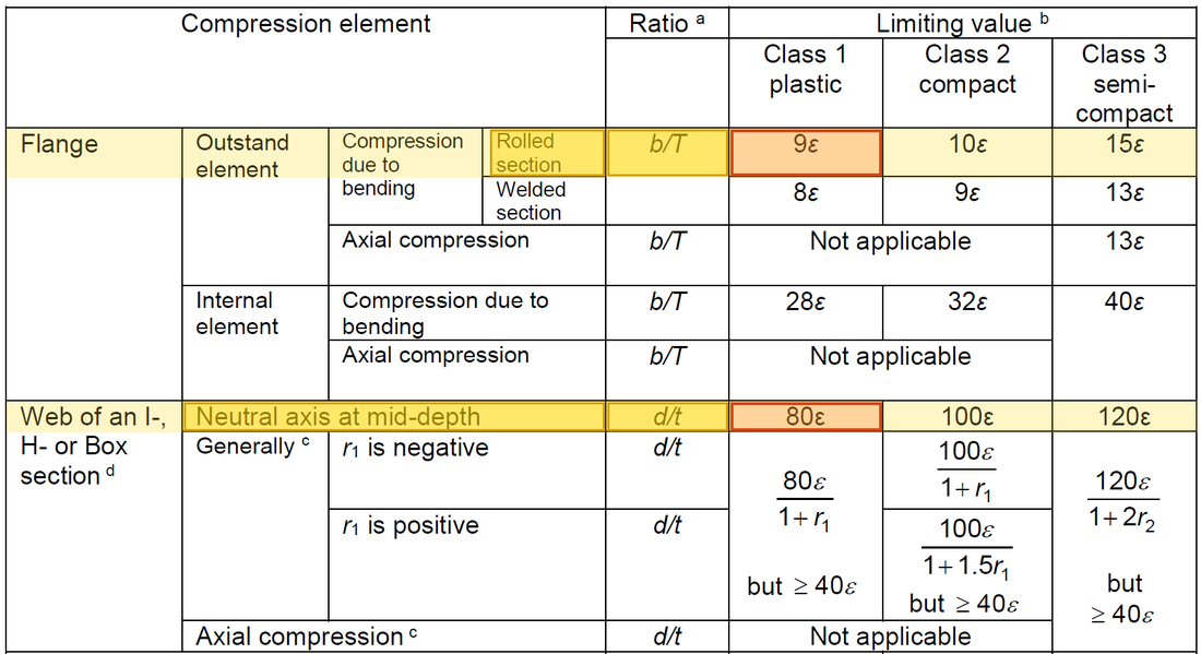
The limits are in terms of ; here , so , 9ε ≈ 8.04 and 80ε ≈ 71.4. and are both within the limits.Yellow: given parameter, row or columnOrange: value read from the table, boxed orange in the text too - Step 10 · AB effective length and LTB
Why this step: Between the two supports nothing holds span AB sideways, so its compressed top flange can bow sideways. measures how prone the span is to this sideways movement and twisting.
Use 7000 mm for AB and the section parameters to obtain and .
New symbols in this step- , : Effective unrestrained length and weak-axis radius of gyration; both in mm
- , : Ordinary and equivalent slenderness; dimensionless
Units: The 7 m span is multiplied by 1000 to give 7000 mm, so it can be divided by in mm. Millimetres divided by millimetres leave slenderness with no unit.
- Step 11 · Tabulated resistance
Why this step: is far below , which shows that this long unrestrained span buckles sideways well before the section reaches its full strength. is the bending capacity that can be relied on for AB.
In the column of Table 8.3a, lies between the 105 and 110 rows; interpolation gives (not ).
New symbols in this step- , , , : Slenderness and table values of the two rows used for interpolation
Where the numbers come from: from Step 10.
Units: is multiplied by 1000 to change cm³ into mm³, and N/mm² times mm³ gives Nmm. Changing Nmm to kNm divides by 1000000, so only a division by 1000 is left in the formula.
Data file lookup · Data Page 5 · Table 8.3a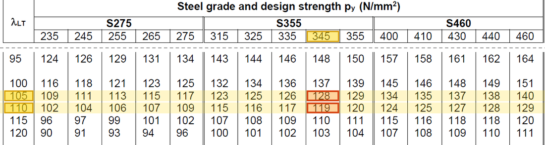
Table 8.3a, column: → 128 and → 119 N/mm²; interpolating at gives .Yellow: given parameter, row or columnOrange: value read from the table, boxed orange in the text too - Step 12 · Obtain the factor from quarter-point moments
Why this step: The quarter-point moments describe how full the moment diagram is. The closer the diagram is to the largest moment along the whole span, the closer is to 1 and the less the demand can be reduced.
, and are the moments at the quarter points of AB (, 3.5 and 5.25 m), from in step 6; the lecturer’s diagram gives 334.8, 392.4 and 312.5 kNm, with .
New symbols in this step- , : Moment-diagram ratio and equivalent moment factor; dimensionless
- Step 13 · AB comparison
Why this step: The equivalent demand is below , so span AB does not move sideways and twist under this load pattern. The two values are close, so the margin is small.
Do not insert the other pattern's 369.9 into this set of quarter-point factors.
New symbols in this step- , : Plastic modulus cm³ or mm³; LTB resistance kNm
AB passes LTB. Overhang BC, other load patterns and serviceability require separate checks; the lecturer does not complete those in class.
All the symbols of this example
| Symbols | Meaning and Units |
|---|---|
| , | Effective unrestrained length and weak-axis radius of gyration; both in mm |
| , | Ordinary and equivalent slenderness; dimensionless |
| , , , | Course LTB section/conversion parameters; dimensionless |
| , | Design yield and bending buckling strengths; N/mm² |
| , | Plastic modulus cm³ or mm³; LTB resistance kNm |
| , | Moment-diagram ratio and equivalent moment factor; dimensionless |
| , , , | Quarter-point and maximum moments from the same load case; kNm |
| , , , | Slenderness and table values of the two rows used for interpolation |
Video positions: 24 October 00:40:00 · 24 October 01:00:00 · 24 October 01:05:00 · 24 October 01:10:00 · 24 October 01:20:00