B3 with midspan restraint: complete the LTB procedure (Restrained Segments)
Task: Distinguish ordinary slenderness , equivalent slenderness , tabulated strength and equivalent moment.
Go straight to Step 1 ↓Design flow for this type of question: Unrestrained beam (lateral-torsional buckling) →
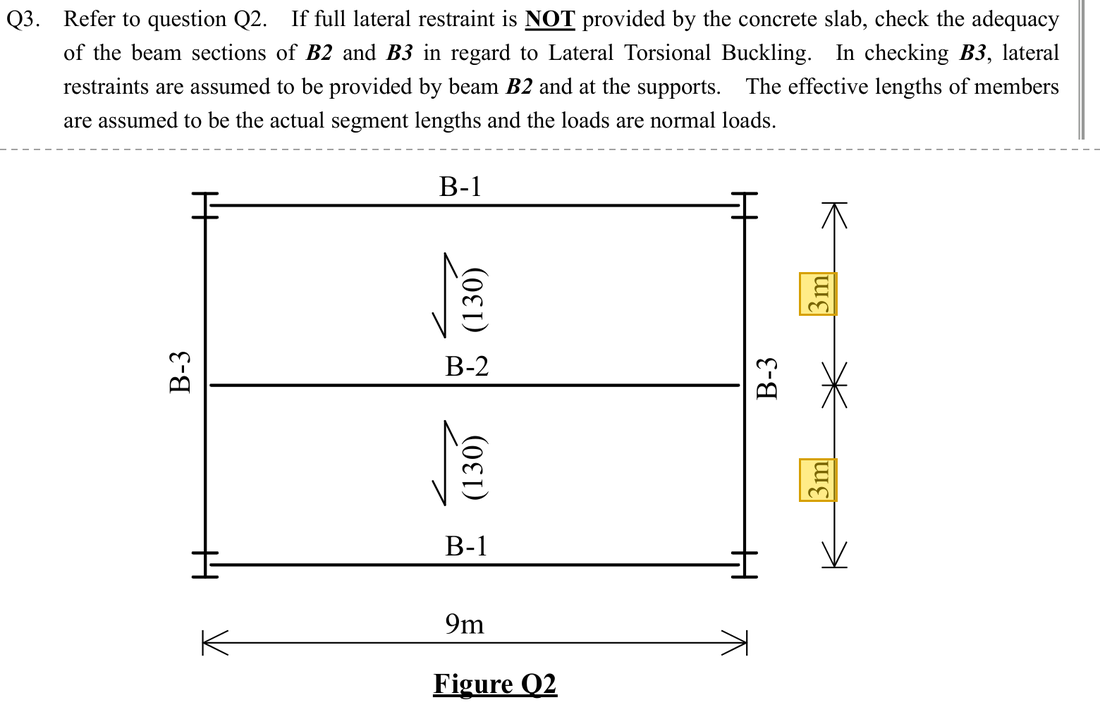
The question in short: Beam B3 is a 457×191×67 UB spanning 6 m. It is held sideways at both ends and at mid-span, so each unrestrained length is 3000 mm. The largest moment is 333.144 kNm. Decide whether this length fails by lateral-torsional buckling.
What differs from the previous example of this type: Same section as B2, but there is now a sideways restraint at mid-span, so the unrestrained length is half the span, not the full span. The moment diagram also differs, so is looked up again.
| Given | Value and Unit |
|---|---|
| Geometry | B3 (457×191×67 UB, S355), span 6 m, laterally restrained at both ends and midspan; this segment |
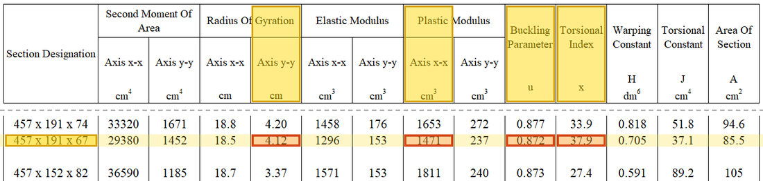
| Section parameters | ; ; ; |
| Classification and strength | Class1/2, ; |
| Bending moment | (B3 example); this segment , |
Yellow: values given in the question. The same values are marked where they are substituted in the steps below.
Orange box: values read directly from the Data File, the same values boxed orange in the lookup screenshots. A value interpolated between two table rows is a calculation, so it has no box.
Solution Route: →→→→→; separately derive from the moment diagram, then compare demand and resistance.
This browser cannot show the 3D model.
Bending puts the top flange in compression, and a compressed flange can buckle sideways like a column. B2 holds the top flange of B3 at midspan, so each segment is only 3 m.
- Largest moment (midspan)333.144 kNm
- Segment between restraints;
- Buckling strength, below
- Lateral-torsional buckling (equivalent moment)Demand 199.8864 kNmCapacity 373.48 kNmUtilisation 0.54
- Step 1 · Define the segment
Why this step: A sideways restraint holds the beam like a hand from the side. The compression flange can only bow sideways between two restraints, so a shorter length makes the beam harder to buckle.
Use the 3 m between adjacent effective lateral restraints, not the full 6 m span .
New symbols in this step- , : Effective unrestrained length and weak-axis radius of gyration; both in mm
- , : Ordinary and equivalent slenderness; dimensionless
Load path · Load, shear force and bending momentGreen marks the lateral restraints: the two supports and B2 at midspan. The top flange can only buckle between restraints, so each segment has an effective length of 3000 mm. In each segment the moment rises from zero at one end to the maximum at the other, so and . - Step 2 · Calculate
Why this step: turns the section's resistance to twisting into a factor below 1. The next step uses it to reduce the ordinary slenderness into the slenderness used for lateral-torsional buckling.
Calculate before squaring. The quarter power is in the denominator, equivalent to raising the whole bracket to −1/4.
New symbols in this step- , , , : Course LTB section/conversion parameters; dimensionless
Where the numbers come from: from Step 1.
- Step 3 · Convert to equivalent slenderness
Why this step: Ordinary slenderness only describes sideways bending, but lateral-torsional buckling also involves twisting. combines both in one value; the smaller it is, the closer the beam gets to using its full section strength.
, and are course-method parameters. This step obtains for the lookup.
- Step 4 · Interpolate within the same strength column
Why this step: is the bending stress this length can carry before it moves sideways and twists. It is lower than ; the difference is the strength lost because the beam may buckle.
In the column, gives 257 and 65 gives 239 N/mm². 60.86 lies between them.
New symbols in this step- , : Design yield and bending buckling strengths; N/mm²
- , , , : Slenderness and table values of the two rows used for interpolation
Where the numbers come from: from Step 3.
Data file lookup · Data Page 5 · Table 8.3a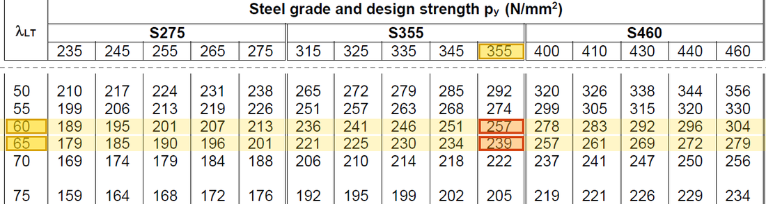
Table 8.3a, column: → 257 and → 239 N/mm²; interpolating at gives .Yellow: given parameter, row or columnOrange: value read from the table, boxed orange in the text too - Step 5 · Resistance units
Why this step: is the largest moment this length can carry before lateral-torsional buckling. It is the capacity in this check and is compared with the demand later.
With supplied in cm³, the conversions simplify to in kNm.
New symbols in this step- , : Plastic modulus cm³ or mm³; LTB resistance kNm
Units: is in N/mm² and in cm³. Multiplying cm³ by 1000 gives mm³, so the product is in Nmm. Changing Nmm to kNm divides by 1000000, so the net step is a division by 1000.
- Step 6 · Demand factor
Why this step: The moment in this length rises from zero at one end to the largest value at the other. Only a short part carries a high moment, which is less severe than the largest moment acting along the whole length.
The segment moment diagram has , giving . Do not multiply resistance by .
New symbols in this step- , : Moment-diagram ratio and equivalent moment factor; dimensionless
- , , , : Quarter-point and maximum moments from the same load case; kNm
Data file lookup · Data Page 6 · Table 8.4a
Table 8.4a: → .Yellow: given parameter, row or columnOrange: value read from the table, boxed orange in the text too - Step 7 · Conclusion
Why this step: Demand below capacity means this length will not move sideways and twist under the design loads. Whether the section itself fails in bending is still a separate check.
199.89<373.48, so this segment passes LTB. The original moment has not physically changed to 199.89; that is the equivalent demand used in this check.
Small differences result from intermediate rounding. Keep the same column throughout; do not interpolate arbitrarily between different strength columns.
All the symbols of this example
| Symbols | Meaning and Units |
|---|---|
| , | Effective unrestrained length and weak-axis radius of gyration; both in mm |
| , | Ordinary and equivalent slenderness; dimensionless |
| , , , | Course LTB section/conversion parameters; dimensionless |
| , | Design yield and bending buckling strengths; N/mm² |
| , | Plastic modulus cm³ or mm³; LTB resistance kNm |
| , | Moment-diagram ratio and equivalent moment factor; dimensionless |
| , , , | Quarter-point and maximum moments from the same load case; kNm |
| , , , | Slenderness and table values of the two rows used for interpolation |
Video positions: 24 October 00:30:00 · 24 October 00:35:00