Pure-compression UC column: from two-axis lookup to capacity (Axial Compression)
Task: Use section dimensions and length to understand why the weak axis governs here.
Go straight to Step 1 ↓Design flow for this type of question: Column: axial force with moments →
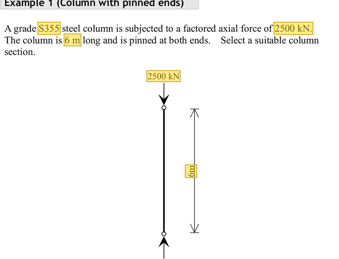
The question in short: S355 steel column is pinned at both ends, with an effective length of 6 m, and carries a compression force of 2500 kN. A 305×305×118 UC is tried. Decide whether the column can carry this force without buckling.
| Given | Value and Unit |
|---|---|
| Problem | S355; pinned at both ends, effective length 6 m; |
| Trial section | 305×305×118 UC; , ; ; ; |
Yellow: values given in the question. The same values are marked where they are substituted in the steps below.
Orange box: values read directly from the Data File, the same values boxed orange in the lookup screenshots. A value interpolated between two table rows is a calculation, so it has no box.

Solution Route: Consistent units→two-axis slenderness →axis-specific curves→compare →capacity versus demand.
The axial force passes straight down the column. The column can buckle about either axis; the more slender axis buckles first and sets the capacity.
- Axial compression
- Buckling about the axis→ pcx ≈ 302 N/mm²
- Buckling about the axis (governs)→ pcy = 193 N/mm²
- Compression buckling capacityDemand 2500 kNCapacity 2895 kNUtilisation 0.86
- Step 1 · Consistent lengths
Why this step: A column can bow in two directions, so slenderness is found for each axis. The direction with the smaller is the thinner one, where the column bows more easily.
Centimetres also work if numerator and denominator agree: 6 m=600 cm.
New symbols in this step- , , , : Effective length and radius of gyration mm; dimensionless slenderness
Units: The 6 m effective length is multiplied by 100 to give 600 cm, the same unit as and . Centimetres divided by centimetres leave slenderness with no unit.
Data file lookup · Data Page 11 · Universal Columns — Dimensions
305×305×118 UC: flange (between 16 and 40 mm).Yellow: given parameter, row or columnOrange: value read from the table, boxed orange in the text too Data file lookup · Data Page 1 · Design strength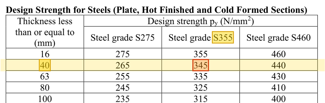
thick: the row, S355 column gives . How the grade and thickness choose this row →Yellow: given parameter, row or columnOrange: value read from the table, boxed orange in the text too - Step 2 · Choose curves
Why this step: is the compressive stress the column can carry before it bows. The more slender the column, the further falls below ; here the weak axis gives a clearly lower .
The lecturer selects each curve from section type, thickness and buckling axis. Do not simply use one curve and change .
New symbols in this step- , , , : Slenderness and table values of the two rows used for interpolation
Where the numbers come from: from Step 1; from Step 1.
Data file lookup · Data Page 7 · Table 8.7 Buckling curves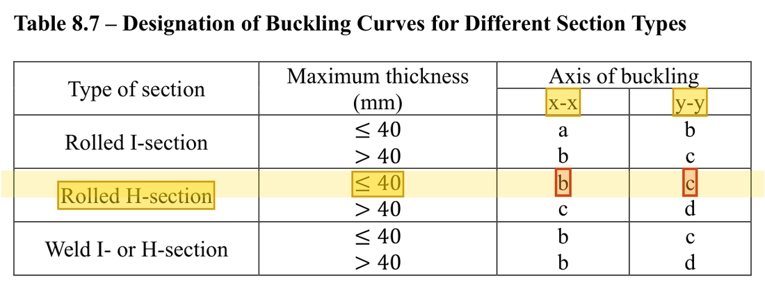
Rolled H-section with thickness ≤ 40 mm: use curve b about the axis and curve c about the axis.Yellow: given parameter, row or columnOrange: value read from the table, boxed orange in the text too Data file lookup · Data Page 8 · Table 8.8(b)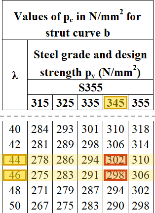
Table 8.8(b) ( axis, curve b), column: → 302 and → 298 N/mm²; gives .Yellow: given parameter, row or columnOrange: value read from the table, boxed orange in the text too Data file lookup · Data Page 8 · Table 8.8(c)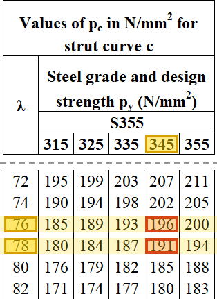
Table 8.8(c) ( axis, curve c), column: → 196 and → 191 N/mm²; interpolating at gives .Yellow: given parameter, row or columnOrange: value read from the table, boxed orange in the text too - Step 3 · Take the governing value
Why this step: The column buckles in whichever direction is easiest, so the smaller decides the result. Here that is the weak axis, so the column would bow about the axis.
The axis lookups give 302 and 193. Use the smaller 193 for governing resistance.
New symbols in this step- , , : Gross area mm²; yield and compression buckling strengths N/mm²
Where the numbers come from: from Step 2.
Load path · A column can buckle about either axisThe same column and the same effective length, but the two axes have different radii of gyration. is smaller, so is larger and buckling about – comes first (red); the compressive strength is the smaller of the two. - Step 4 · Convert area
Why this step: is the largest compression force the whole column can carry before it bows: the stress each square millimetre can take, multiplied by the full area of the section.
150 cm²=15000 mm². This conversion is easily missed.
New symbols in this step- , : Design axial force and buckling compression resistance; kN
Where the numbers come from: from Step 2.
Units: The area of 150 cm² is multiplied by 100 to change it into mm². N/mm² times mm² gives N, and dividing by 1000 gives kN.
- Step 5 · Comparison
Why this step: A ratio below 1 means the design force is not enough to make the column bow. The part left over is the margin of safety.
Resistance exceeds design axial force .
Where the numbers come from: from Step 4.
Pure-compression buckling passes. Adding bending requires the relevant interaction expressions; versus alone is then insufficient.
All the symbols of this example
| Symbols | Meaning and Units |
|---|---|
| , | Design axial force and buckling compression resistance; kN |
| , , | Gross area mm²; yield and compression buckling strengths N/mm² |
| , , , | Effective length and radius of gyration mm; dimensionless slenderness |
| , , , | Slenderness and table values of the two rows used for interpolation |
Video positions: 24 October 02:15:00 · 24 October 02:25:00 · 24 October 03:00:00