Beams: loads, section checks and lateral stability
1. Supports vs lateral restraints: two different things Always examined
Simple explanation: A support stops only certain movements
Holding a ruler up does not necessarily stop it sliding sideways or twisting.
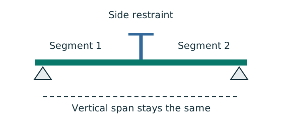
- Identify vertical support, lateral restraint and torsional restraint separately.
- Find which flange is in compression in each region.
- Use only restraints actually provided by the question.
Remember: An extra side restraint does not create a new vertical reaction.
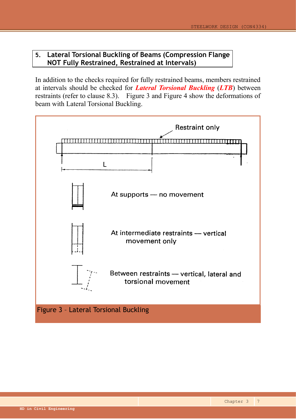
A vertical support stops the beam moving up or down. A lateral restraint stops the compression flange moving sideways. A torsional restraint stops the section twisting. These are not the same: a beam can sit firmly on two supports and still buckle sideways between them. Which flange is compressed depends on the moment: in sagging (the beam bends downwards) the top flange is compressed; in hogging (e.g. a cantilever) the bottom flange is compressed.
The course counts a restraint as effective if it can resist of the largest design force in the compression flange; a concrete slab normally can. So if the question says “fully restrained”, there is no LTB check, but you still check shear, bending, the web (if asked) and deflection. If restraints are only at certain points, check LTB for every segment. A point load on its own is not a restraint.
Try it yourself. A beam has lateral restraints at , , and . Is it three independently simply supported vertical beams?
Reveal answer and reasoning
No. Vertical bending analysis still uses the actual vertical supports. The three lengths are the LTB segments; internal moments at the lateral restraints are generally nonzero.
Concept map: Lateral-torsional buckling: why does a beam tip over sideways?
Concept map
Lateral-torsional buckling: why does a beam tip over sideways?
Understand the mechanism and the LTB calculation starts to make sense: every formula measures how easily the compression flange can escape sideways. The mechanism runs down the middle, with what makes it worse and how design responds.
- Cause
- Key idea
- Result
- What changes it
- How design deals with it
- Exam answer
- marks are often lost here
Text version (from cause to result)
Cause
The beam bends
In sagging the top flange is compressed and the bottom flange stretched; in hogging (e.g. a cantilever) the bottom flange is compressed.
Comes from (upstream)— (a starting point)
Leads to (downstream)The compression flange acts like a slender strut
Key idea
The compression flange acts like a slender strut
The compressed flange behaves like a slender strut that wants to bow sideways — about the weak axis of the section.
Comes from (upstream)The beam bends
Leads to (downstream)It bows sideways and twists
Key idea
It bows sideways and twists
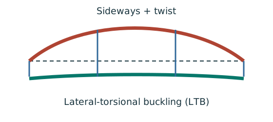
The tension flange wants to stay straight while the compression flange moves sideways, so the whole section moves sideways and twists. That is lateral-torsional buckling.
Comes from (upstream)The compression flange acts like a slender strut
Leads to (downstream) Fails before the section is fully used
How design deals with itWhere marks are lost
Lateral restraint (×): holds the compression flange at the side
Restraints split the beam into segments; shorter segments are safer. A restraint counts if it can resist 2.5% of the largest compression-flange force.
Comes from (upstream)— (a starting point)
Leads to (downstream) Longer unrestrained lengthA slab holds it all along → no LTB check
Result
Fails before the section is fully used
The beam fails sideways before reaching its section moment capacity , so it is checked against the smaller .
Comes from (upstream)It bows sideways and twists
Leads to (downstream) Restrained at a few points → check each segment
What changes it
Longer unrestrained length
The longer the flange is free between lateral restraints, the more easily it bows out. With normal loads is the segment length.
Comes from (upstream)Lateral restraint (×): holds the compression flange at the side
Leads to (downstream) Restrained at a few points → check each segment
What changes it
Weak-axis stockiness
The smaller (the narrower the flange), the easier it bows sideways. A narrow-flanged UB is more prone to LTB than a UC.
Comes from (upstream)— (a starting point)
Leads to (downstream) Restrained at a few points → check each segment
What changes it
Load on the top flange that moves with it
Once the beam twists, the load pushes it over further (destabilizing load), so . Exam questions usually state “normal load”.
Comes from (upstream)— (a starting point)
Leads to (downstream) Restrained at a few points → check each segment
What changes it
Shape of the moment diagram
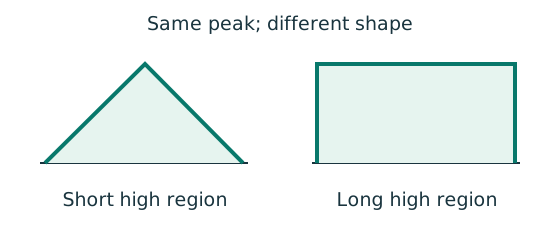
A segment near the peak moment all along is most dangerous; a single peak is less so. turns an uneven moment into an equivalent uniform one.
Comes from (upstream)— (a starting point)
Leads to (downstream) Restrained at a few points → check each segment
How design deals with it
A slab holds it all along → no LTB check
A slab restrains the beam along its whole length (full lateral restraint), so the compulsory floor beams need no LTB check — but still need shear, bending and deflection.
Comes from (upstream)Lateral restraint (×): holds the compression flange at the side
Leads to (downstream)Exam: tell supports from restraints first
How design deals with it
Restrained at a few points → check each segment
All the factors above end up in one check: and → → → ; the moment shape → . Steps: LTB calculation map.
Comes from (upstream) Fails before the section is fully used Longer unrestrained length Weak-axis stockinessLoad on the top flange that moves with it Shape of the moment diagram
Leads to (downstream)Exam: tell supports from restraints first
Exam answer
Exam: tell supports from restraints first
On the drawing: triangle / roller = support (reaction); cross × = lateral restraint (no reaction, only splits segments). “Fully restrained” means no LTB check.
Comes from (upstream)A slab holds it all along → no LTB check Restrained at a few points → check each segment
Leads to (downstream)— (the last step)
Tour steps
1. The compression flange is a strut
The beam bends → one flange is compressed → like a slender column it wants to bow sideways.
In this stepThe beam bendsThe compression flange acts like a slender strut
2. Sideways plus twist
The tension flange does not follow, so the section moves sideways and twists, failing before .
In this stepIt bows sideways and twists Fails before the section is fully used
3. What makes it worse?
A long unrestrained length, a slim weak axis, load on the top flange, and a segment near the peak moment all along.
In this step Weak-axis stockinessLoad on the top flange that moves with it Shape of the moment diagram
4. The remedy: lateral restraint
Hold the compression flange at the side to shorten the unrestrained length. A slab holding it all along → no LTB check.
In this stepLateral restraint (×): holds the compression flange at the side Longer unrestrained lengthA slab holds it all along → no LTB check
5. Everything ends in one check
Everything becomes , written once per segment.
In this step Restrained at a few points → check each segment
6. The first exam step
First separate supports from lateral restraints on the drawing — the most common mistake starts here.
In this stepExam: tell supports from restraints first
Animation labA beam bends sideways and twists
Supplement to the original lesson. Enable JavaScript to play, step through calculations and rotate 3D models. The following explanation remains readable offline.
- For the illustrated sagging beam the top flange is compressed.
- The unrestrained compression flange can move sideways while the complete cross-section twists.
- Only effective restraints divide the member into unbraced segments. They do not automatically add vertical supports.
- Use the segment effective length, section properties and matching moment factor. This is an exaggerated mode shape, not a calculated displacement.
2. Shear capacity : can the web take it? Always examined
Simple explanation: What shear is trying to do
Imagine cutting the beam: shear stops the two cut faces sliding past each other.
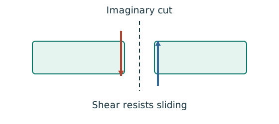
- Find the design shear from the load analysis.
- Use the section’s applicable shear area and strength.
- Compare demand with resistance in the same force units.
Remember: The web usually carries much of the vertical shear in an I-section.
| Section / load direction | Shear area |
|---|---|
| Rolled I, H or channel, load parallel to web | |
| Welded I, load parallel to web | |
| Rectangular hollow section | |
| T section | |
| Circular hollow section | |
| Solid rectangle | |
| Other section | , where is the relevant rectilinear element area |
Symbols: overall depth, clear web depth (between the root fillets), web thickness, flange thickness. Exam sections are hot-rolled, so . If (), the web will not wrinkle in shear and the formula above applies directly — but that does not excuse the web bearing and web buckling checks at a support (sections 5 and 6). Finally compare the largest shear in the beam (ignoring its sign) with .
Animation labSee shear in the web
Supplement to the original lesson. Enable JavaScript to play, step through calculations and rotate 3D models. The following explanation remains readable offline.
- Internal shear keeps the two sides of the cut in vertical equilibrium.
- For the course’s common I-section case, the web provides the principal shear area; use the specified definition.
- A slender web may require a different shear-buckling route before a simple shear-resistance formula is used.
- Use where applicable in the course. Convert N to kN before comparing with design shear.
3. Moment capacity (low shear) Always examined
Simple explanation: Why one flange squeezes and the other stretches
Bending makes opposite sides of the section do opposite jobs.
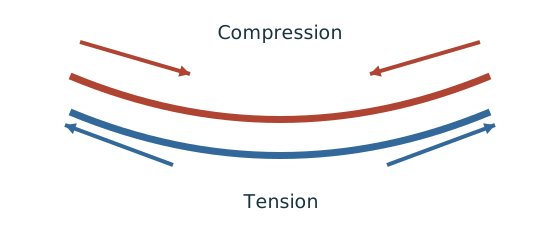
- Find the moment from the actual loads and supports.
- Choose the resistance formula allowed by the section class.
- Check whether the coexistent shear changes that formula.
Remember: Use shear at the location being checked, not an unrelated maximum.
First find the section class from the flange and web ratios; take the worse one. Then look at the shear where you are checking: if (low shear — almost always in exams), use the formulas in the table below. is the plastic modulus, the elastic modulus. Unit shortcut: .
| Class | Low-shear moment resistance |
|---|---|
| 1 plastic or 2 compact | |
| 3 semi-compact | pᵧZ, or pᵧSₑff where the permitted effective plastic property is established |
| 4 slender | pᵧZₑff or pᵧᵣZ, using an established effective property/reduced strength |
is the course’s cap that stops the beam yielding too early under normal loads. In the check , is the actual largest moment (not the LTB value , which belongs to a different check). Class 3 may only use ; Class 4 needs effective properties and does not occur with the usual exam sections.
Animation labCompression and tension across a section
Supplement to the original lesson. Enable JavaScript to play, step through calculations and rotate 3D models. The following explanation remains readable offline.
- For sagging, the top flange is in compression and the bottom in tension; hogging reverses this.
- Elastic bending stress varies with distance from the neutral axis: .
- The section class governs whether elastic, plastic or effective properties may be used.
- Use the shear at the section under examination; the largest shear elsewhere is not automatically coexistent.
4. When shear is high, the moment capacity drops Background
Simple explanation: The web is doing two jobs
Heavy shear leaves less of the web’s strength available for bending.
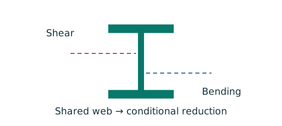
- Check the course trigger using the coexistent shear.
- If triggered, use the appropriate reduced bending expression.
- Recheck moment demand against the reduced resistance.
Remember: The reduction is conditional; do not apply it to every beam.
Use these formulas only when the shear at the same position is above . is the plastic modulus of the shear area (the web rectangle), not of the whole section: for a rectangle wide and deep, . If , the shear check has already failed; choose a bigger section.
Try it yourself. . What is ?
Reveal answer and reasoning
. Reduce the bending contribution associated with the shear area; do not reduce the entire section capacity by .
Animation labHigh shear reduces bending resistance
Supplement to the original lesson. Enable JavaScript to play, step through calculations and rotate 3D models. The following explanation remains readable offline.
- Part of the web contributes to bending while also carrying shear.
- The course low-shear route applies at . Above it, follow the applicable reduction expression.
- The highlighted web contribution is reduced, not the complete cross-section by an arbitrary percentage.
- Retain the section-class-specific formula and all bounds shown in the original calculation.
Animation labHigh shear reduces bending resistance
Supplement to the original lesson. Enable JavaScript to play, step through calculations and rotate 3D models. The following explanation remains readable offline.
- Part of the web contributes to bending while also carrying shear.
- The course low-shear route applies at . Above it, follow the applicable reduction expression.
- The highlighted web contribution is reduced, not the complete cross-section by an arbitrary percentage.
- Retain the section-class-specific formula and all bounds shown in the original calculation.
5. Web bearing: can a point force crush the web? Background
Simple explanation: A concentrated force can hurt one small region
A narrow contact presses much harder locally than the same force spread over a wider contact.
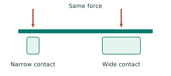
- Find the actual stiff bearing length and end position.
- Check local crushing and local web buckling separately.
- Use the restraint conditions required by each expression.
Remember: Missing contact dimensions cannot be guessed from drawing scale.
The force spreads down through the flange before entering the web. is the stiff bearing length — the part of the bearing that does not bend noticeably, which is not always the full plate width. Measure it from the matching lecture sketch, or use the given in the question.
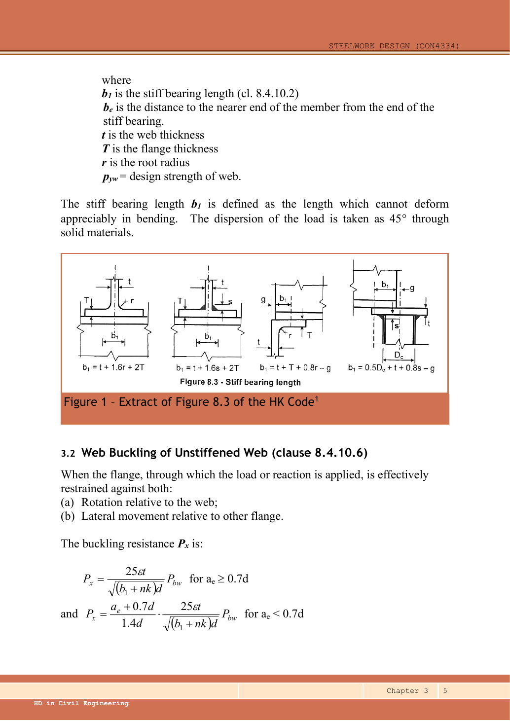
is the root radius; is the distance from the edge of the bearing to the beam end; is the design strength of the web. With all lengths in mm, comes out in N (÷1000 for kN); compare it with the design reaction there. Without or it cannot be calculated.
Animation labSpread a concentrated force into the web
Supplement to the original lesson. Enable JavaScript to play, step through calculations and rotate 3D models. The following explanation remains readable offline.
- A concentrated reaction first enters through the bearing/contact region.
- The flange and root geometry spread the force before it enters the web.
- A wider effective bearing region can reduce local stress for the same force.
- End distance, stiff bearing length and restraint conditions must come from the original question. This slider is illustrative only.
6. Web buckling: the web bows like a short column Background
Simple explanation: What to do when one input is missing
A calculator cannot supply a dimension that the drawing never gave.
- Separate given values, table values and calculated values.
- Complete the checks whose required inputs are available.
- State the missing input beside the remaining conditional result.
Remember: An illustrative assumption must not become an unstated exam given.
First confirm the loaded flange is restrained (it cannot rotate relative to the web or move sideways relative to the other flange). If both hold, use below. is the distance from the load (reaction) line to the beam end; is measured from the edge of the bearing — they are different.
Both multipliers have no units. If the flange is not restrained, reduce further by ( is the effective length of the web as a strut, not the beam’s LTB length). Compare with the same concentrated force as in section 5. Passing the shear check does not mean this one passes.
Try it yourself. is centred on a bearing that starts at the member end. What are and ?
Reveal answer and reasoning
; . The first is measured to the bearing edge, the second to the centred reaction line.
Animation labThe web behaves like a short strut
Supplement to the original lesson. Enable JavaScript to play, step through calculations and rotate 3D models. The following explanation remains readable offline.
- A concentrated force compresses a local region between the flanges.
- The thin web can buckle sideways before local crushing governs.
- The source distinguishes restraint against rotation and relative lateral movement.
- Web bearing and web buckling are separate checks. Select the original expression whose assumptions are satisfied.
Animation labThe web behaves like a short strut
Supplement to the original lesson. Enable JavaScript to play, step through calculations and rotate 3D models. The following explanation remains readable offline.
- A concentrated force compresses a local region between the flanges.
- The thin web can buckle sideways before local crushing governs.
- The source distinguishes restraint against rotation and relative lateral movement.
- Web bearing and web buckling are separate checks. Select the original expression whose assumptions are satisfied.
7. Full procedure for a fully restrained beam (compulsory question) Always examined
Simple explanation: How a floor load reaches a beam
Each beam collects the load from its own strip of floor.
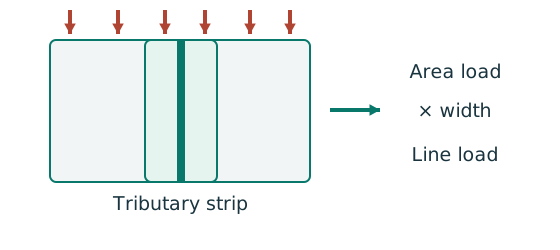
- Find the tributary width from the actual plan.
- Area load × tributary width gives load per beam length.
- A supporting beam receives the other beam’s end reaction.
Remember: A reaction becomes a point load, not automatically a UDL.
Simple explanation: How much does the beam sag?
Strength asks whether it fails; deflection asks how far it moves.
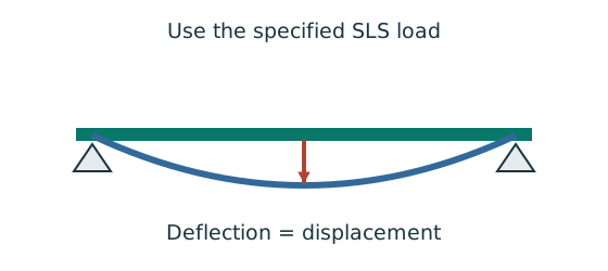
- Use the serviceability load case specified by the course question.
- Choose the expression matching the support and load positions.
- Use consistent units for load, length, E and I.
Remember: The largest deflection is not always at midspan.
- Draw the load path: slab → secondary beam → main beam. Area load (kN/m²) × tributary width (m) = line load (kN/m); the reactions of supported beams become point loads on the main beam.
- Keep dead and imposed loads separate. Beam self-weight = mass × ÷ 1000, added once (not again if the question says it is included).
- Apply the factors (1.4, 1.6) and use equilibrium for reactions, shear and moment; the maximum moment is where the shear is zero (or changes sign).
- If you must choose a section: estimate , pick a section from the table, then confirm with its flange thickness.
- Classify, then check shear, bending at low shear, and any web bearing or buckling the question asks for.
- Check deflection with the unfactored imposed load. If anything fails, choose a bigger section and redo the affected checks.
Deflection uses the unfactored imposed load and ; with brittle finishes the limit is (lecture examples 1 and 2 assume brittle finishes). Use the stated limit for other cases (ordinary beams , cantilevers ).
Work in N, mm and mm⁴: , . These two formulas apply only to a simply supported beam with a full-span UDL and a midspan point load; off-centre loads, cantilevers and continuous beams need their own working (see example 3).
Understanding map: Compulsory floor beams: load flows from the slab to B1, then to B2
Understanding map
Compulsory floor beams: load flows from the slab to B1, then to B2
This map is the load path: the slab’s weight lands on B1, and B1’s end reaction becomes the load on B2. Notice the two routes: factored design loads (for strength) and unfactored imposed load (for deflection). The values are from 2024 Q1.
- From the question
- From the tables
- Worked out
- Demand
- Capacity
- Check
- marks are often lost here
Text version (in working order)
From the questionWhere marks are lost
Slab
Slab thickness (in m) × concrete density 24.5 kN/m³, plus finishes 0.4 kN/m².
Needs (upstream)— (a starting value)
Used for (downstream) Dead load per m²
From the question
Imposed load
Imposed load per m² (kN/m²). It takes two routes: × 1.6 for strength, unfactored for deflection.
Needs (upstream)— (a starting value)
Used for (downstream) Design area load Imposed line load (unfactored)
Worked out
Dead load per m²
Slab self-weight plus finishes.
Formula
2024 Q1
Needs (upstream) Slab
Used for (downstream) Design area load
From the question
B1 tributary width
An interior B1 takes half the spacing on each side: . An edge beam takes one side only.
Where it comes from: The beam spacing on the floor plan.
Needs (upstream)— (a starting value)
Used for (downstream) B1 design line load Imposed line load (unfactored)
From the tablesWhere marks are lost
B1 self-weight
Table mass (kg/m) × ÷ 1000 → kN/m. 39.1 kg/m → 0.391 kN/m.
Needs (upstream)— (a starting value)
Used for (downstream) B1 design line load
Demand
Design area load
The answer to (a)(i): dead × 1.4, imposed × 1.6.
Formula
2024 Q1
Needs (upstream) Dead load per m² Imposed load
Used for (downstream) B1 design line load
From the questionWhere marks are lost
B1 span
The length of B1 between its supports (the B2 beams).
Needs (upstream)— (a starting value)
Used for (downstream) B1 shear = end reaction B1 maximum moment Imposed reaction on B2 B1 deflection B1: four checks
From the tables
B2 self-weight
406×140×46 UB: 46 kg/m → 0.46 kN/m.
Needs (upstream)— (a starting value)
Used for (downstream) B2 self-weight (design)
Demand
B1 design line load
The area load times the tributary width becomes load per metre of beam, plus the self-weight × 1.4. (Same as .)
Formula
2024 Q1
Needs (upstream) Design area load B1 tributary width B1 self-weight
Used for (downstream) B1 shear = end reaction B1 maximum moment
Worked outWhere marks are lost
Imposed line load (unfactored)
Deflection uses imposed load only, unfactored. This is where the second route starts.
2024 Q1
Needs (upstream) Imposed load B1 tributary width
Used for (downstream) Imposed reaction on B2 B1 deflection
From the question
B2 span
The length of B2 between its columns.
Needs (upstream)— (a starting value)
Used for (downstream) B2 shear B2 maximum moment B2 deflection B2: four checks
From the tables
Design strength and class
Both flanges are thinner than 16 mm → 355; both beams are Class 1 (part (a)(iv)).
Where it comes from: Core skills: and classification
Needs (upstream)— (a starting value)
Used for (downstream), B1 capacities, B2 capacities
Demand
B1 shear = end reaction
For a simply supported beam the maximum shear is the end reaction. That reaction presses on B2 — the key step of the load path.
Formula
2024 Q1
Needs (upstream) B1 design line load B1 span
Used for (downstream) B2 shear B2 maximum moment B1: four checks
DemandWhere marks are lost
B2 self-weight (design)
B2’s only UDL is its own self-weight × 1.4; the slab load already arrives through B1, so do not count it again.
Formula
2024 Q1
Needs (upstream) B2 self-weight
Used for (downstream) B2 shear B2 maximum moment
Worked out
Imposed reaction on B2
The imposed-load reaction B1 passes to B2, also unfactored.
Formula
2024 Q1
Needs (upstream) Imposed line load (unfactored) B1 span
Used for (downstream) B2 deflection
Demand
B1 maximum moment
For a simply supported beam with a UDL, the maximum moment is at midspan.
Formula
2024 Q1
Needs (upstream) B1 design line load B1 span
Used for (downstream) B1: four checks
DemandWhere marks are lost
B2 shear
B2 receives B1’s reaction at midspan (already factored).
Formula
2024 Q1
Needs (upstream) B1 shear = end reaction B2 self-weight (design) B2 span
Used for (downstream) B2: four checks
Demand
B2 maximum moment
The midspan point load plus the self-weight.
Formula
2024 Q1
Needs (upstream) B1 shear = end reaction B2 self-weight (design) B2 span
Used for (downstream) B2: four checks
DemandWhere marks are lost
B1 deflection
Midspan deflection under the imposed UDL. , .
Formula
2024 Q1
Needs (upstream) Imposed line load (unfactored) B1 span
Used for (downstream) B1: four checks
Demand
B2 deflection
Deflection under the midspan imposed point load. .
Formula
2024 Q1
Needs (upstream) Imposed reaction on B2 B2 span
Used for (downstream) B2: four checks
CapacityWhere marks are lost
, B1 capacities
Shear is carried by the web; the moment capacity is the smaller of and .
Formula
2024 Q1
Needs (upstream) Design strength and class
Used for (downstream) B1: four checks
Capacity
, B2 capacities
The same formulas as B1, with the 406×140×46 UB data.
2024 Q1
Needs (upstream) Design strength and class
Used for (downstream) B2: four checks
Check
B1: four checks
Shear, low shear, bending and deflection — finish each with “… < … ∴ OK”.
2024 Q1
Needs (upstream) B1 shear = end reaction B1 maximum moment, B1 capacities B1 deflection B1 span
Used for (downstream)— (the final conclusion)
Check
B2: four checks
The same four checks; the deflection limit uses B2’s own span.
2024 Q1
Needs (upstream) B2 shear B2 maximum moment, B2 capacities B2 deflection B2 span
Used for (downstream)— (the final conclusion)
Tour steps
1. Read the floor plan
Separate the spans of B1 (secondary) and B2 (main), and work out B1’s tributary width.
In this step B1 tributary width B1 span B2 span
2. (a)(i) Slab design load (4 marks)
, then .
In this step Slab Imposed load Dead load per m² Design area load
3. (a)(ii) B1 load, shear and moment
Area load × tributary width + self-weight → load per metre; then and .
In this step B1 self-weight B1 design line load B1 shear = end reaction B1 maximum moment
4. (a)(iii) B1’s reaction becomes B2’s load
Follow the arrows: flows straight into and . B2 adds only its own self-weight × 1.4.
In this step B2 self-weight B2 self-weight (design) B2 shear B2 maximum moment
5. (a)(iv)–(vi) Capacities
Settle and the class once; both beams use the same formulas for and .
In this step Design strength and class, B1 capacities, B2 capacities
6. Deflection: the unfactored route
Start again from : for B1’s deflection; B1’s imposed reaction for B2’s.
In this step Imposed line load (unfactored) B1 deflection Imposed reaction on B2 B2 deflection
7. Write the conclusions
Each beam needs “… < … ∴ OK” for all four checks. Numbers without a conclusion lose marks.
In this step B1: four checks B2: four checks
Beam example 1: fully restrained beam, from loads to deflection
Open this example on its own page
Select a Grade S355 section for a fully laterally restrained, simply supported beam. Check shear, bending, support web bearing, support web buckling and deflection. The central loads are dead and imposed; full-span UDLs are dead and imposed.
Original source: LectureNotes/Ch 3_Beam.pdf — p. 18, p. 19, p. 20, p. 21. Values tagged given are in the question or diagram; lookup values come from a named table; calculated values follow from the working; assumptions are stated explicitly.
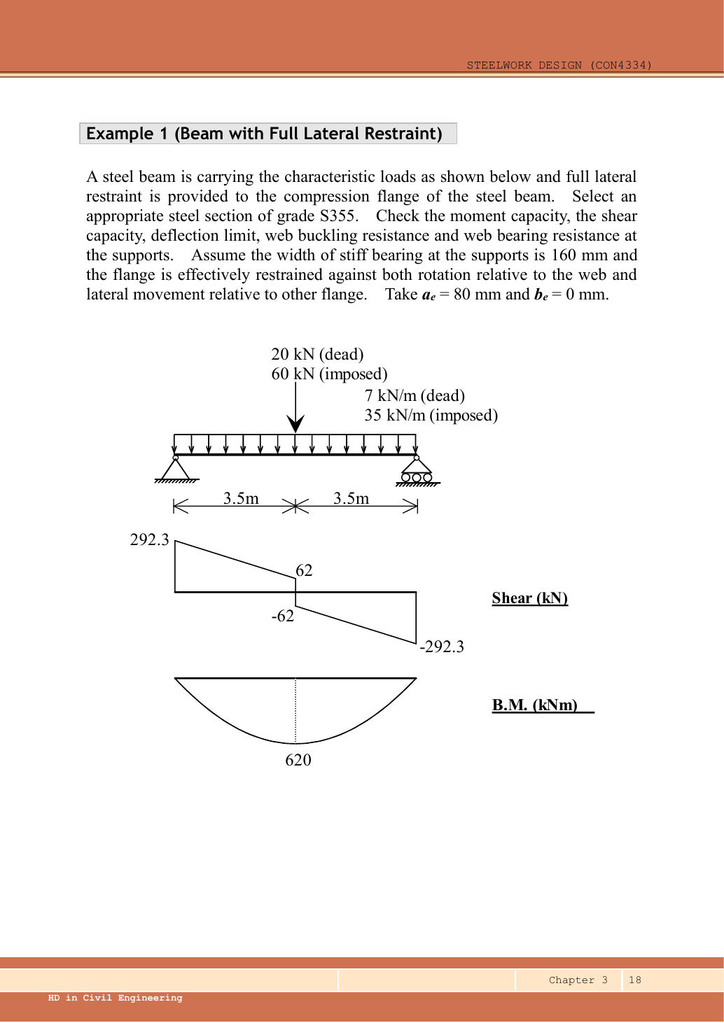
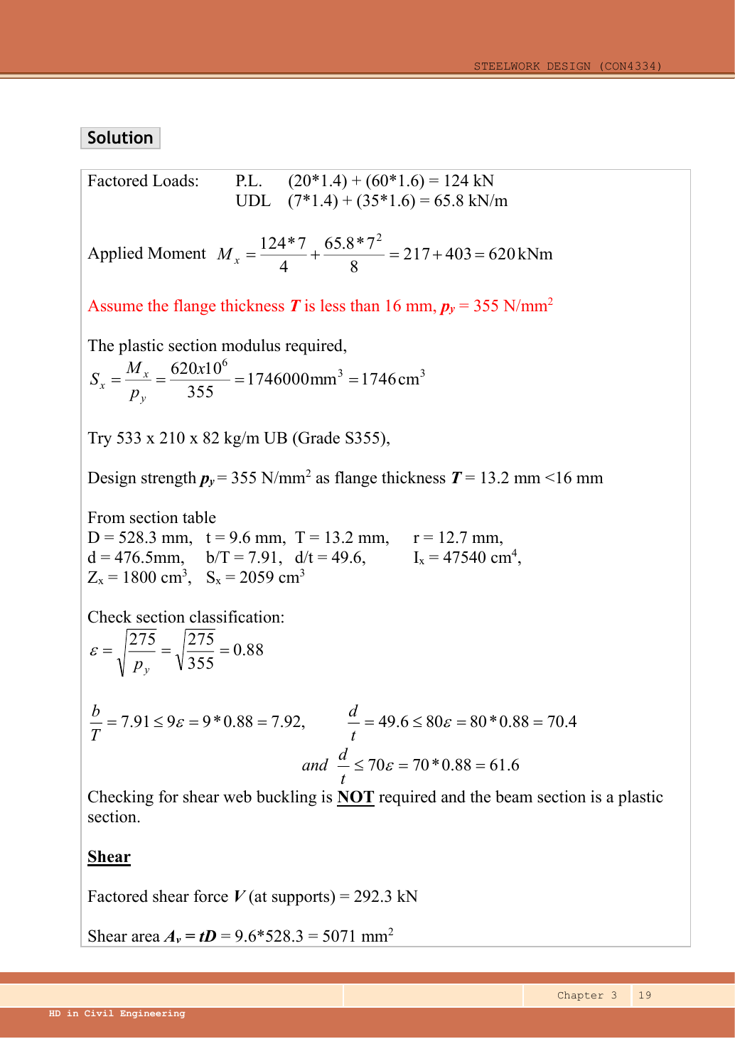
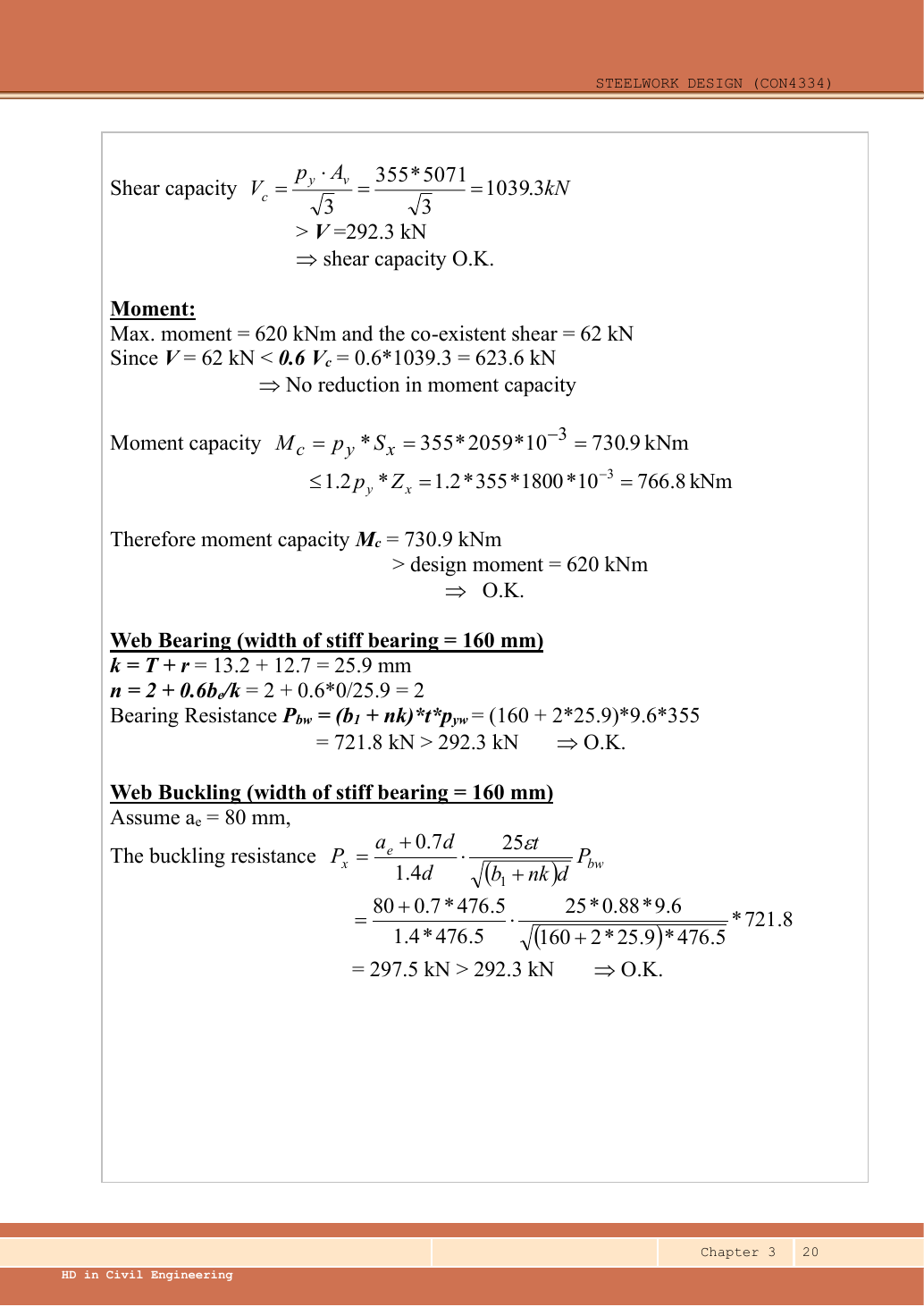
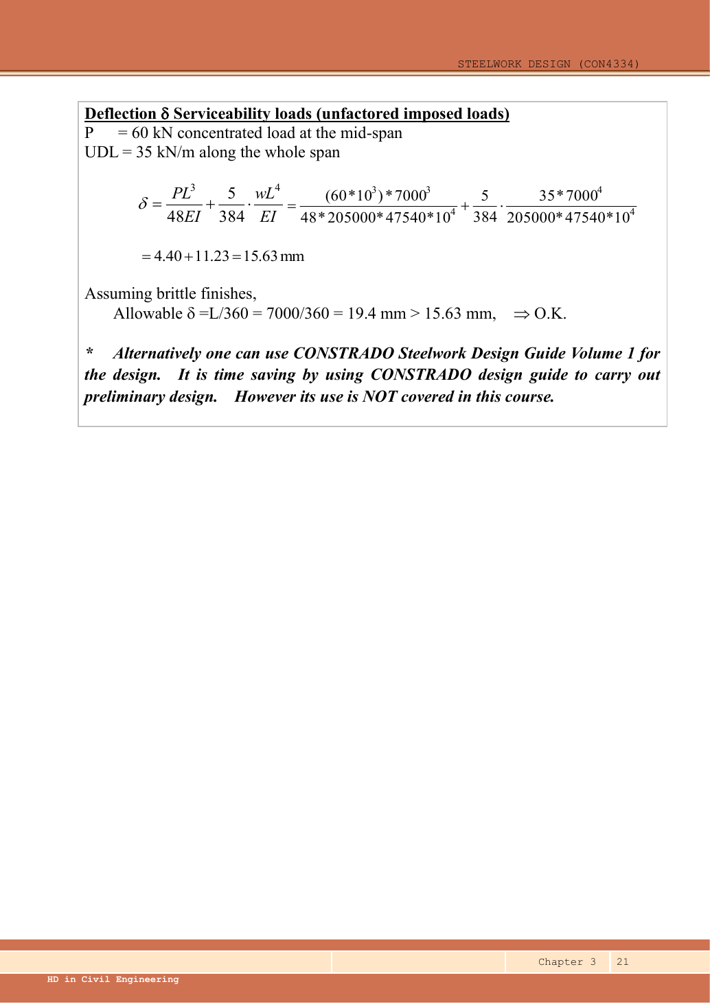
Read the diagram and collect the data
| Quantity | Given, lookup or assumption |
|---|---|
| Span and loading | Given in the upper drawing: , one central point load and two full-span UDL components. |
| Bearing | Given in the question: , , . Loaded flange is restrained against both specified local movements. |
| Lateral restraint | Given: compression flange fully restrained, so no member LTB check is needed. |
| Deflection | Lecturer assumes brittle finishes and uses unfactored imposed loads only; limit . . |
| Section properties | Lookup Data File pp.9–10, row UB. Original solution also lists the values on p.19. |
Before calculating: recognition and strategy
Learn the difference between a load and an action first: load is applied to the beam; shear and moment are internal actions needed to carry it. Symmetry makes the two reactions equal. The shear changes sign at the central point load, so that is the maximum-moment position. Full lateral restraint removes LTB from this example, but does not remove local web checks. Select a trial section from its plastic modulus, then verify every other requirement.
1. Factor each load component
Simple explanation: How a floor load reaches a beam
Each beam collects the load from its own strip of floor.
- Find the tributary width from the actual plan.
- Area load × tributary width gives load per beam length.
- A supporting beam receives the other beam’s end reaction.
Remember: A reaction becomes a point load, not automatically a UDL.
The given dead UDL is the prescribed design input. Do not add an extra assumed self-weight on top of it. Keep the unfactored imposed loads and for the separate deflection calculation.
Animation labFrom characteristic to design load
Supplement to the original lesson. Enable JavaScript to play, step through calculations and rotate 3D models. The following explanation remains readable offline.
- G is permanent load; Q is imposed load. A surface load and a line load also have different units.
- This illustration uses the course gravity case . Other combinations in the original text retain their own factors.
- For illustrative , change Q and watch each separate contribution.
- Do not carry this ULS total automatically into deflection. Follow the stated SLS load case.
2. Reactions, shear and maximum moment
Equivalently . The source labels after rounding. UDL makes shear linear and bending parabolic; the point load makes a shear jump of but no moment jump.
Animation labBalance reactions and moments
Supplement to the original lesson. Enable JavaScript to play, step through calculations and rotate 3D models. The following explanation remains readable offline.
- This demonstrator is a simply supported 6 m beam with a 60 kN point load; it is not the page’s original loading diagram.
- . Moving the load towards B increases .
- . The two upward reactions must sum to P.
- With the load at midspan, . End couples, UDLs and overhangs require their own equilibrium terms.
3. Select a trial section and read the correct columns
| Table column | Selected-row value |
|---|---|
| ; web ; flange ; root ; clear web () | |
| Flange ; web | |
| Major-axis ; elastic ; plastic |
and are nominal section designations, not the exact and flange width. The table’s confirms the initial assumption. Select the major-axis columns because the vertical load bends the beam about . This is the lecturer’s suitable trial section, not a demonstrated minimum-mass optimum.
Animation labRead a table without losing the keys
Supplement to the original lesson. Enable JavaScript to play, step through calculations and rotate 3D models. The following explanation remains readable offline.
- Name the required property: material strength, section property, buckling strength or a moment factor.
- Keep section size, steel grade, thickness band, curve and axis as separate lookup keys.
- , and require different conversion powers. Do not use adjacent columns interchangeably.
- Use bracketing rows within the same valid column. The original page remains the source of all table values.
4. Establish the section class and web-shear branch
Simple explanation: A thin part can wrinkle first
A thin plate may wrinkle before the whole steel member reaches its intended resistance.
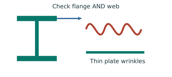
- Check flange and web slenderness using their own definitions.
- Compare each ratio with the correct class limits.
- The less favourable element determines the section class.
Remember: Bending limits and uniform-compression limits are different.
The flange classification is close to its limit: use the table ratio and keep enough precision. The web’s bending-class limit and shear-buckling threshold are different tests. A separate shear-web-buckling calculation is not required; concentrated reaction web buckling is still checked below.
Animation labWhy thin elements buckle locally
Supplement to the original lesson. Enable JavaScript to play, step through calculations and rotate 3D models. The following explanation remains readable offline.
- The flange outstand and web have different widths, thicknesses and edge support conditions.
- A thinner plate can wrinkle locally before the complete member loses stability.
- Class 1 allows plastic rotation; Class 2 reaches plastic resistance; Class 3 reaches elastic resistance; Class 4 requires effective properties.
- Check every relevant compression element with the supplied limits and stress distribution. The deformation shown is qualitative.
5. Resist the largest shear
Animation labSee shear in the web
Supplement to the original lesson. Enable JavaScript to play, step through calculations and rotate 3D models. The following explanation remains readable offline.
- Internal shear keeps the two sides of the cut in vertical equilibrium.
- For the course’s common I-section case, the web provides the principal shear area; use the specified definition.
- A slender web may require a different shear-buckling route before a simple shear-resistance formula is used.
- Use where applicable in the course. Convert N to kN before comparing with design shear.
6. Check coexistent shear, then bending
The largest shear actually also lies below , so every section is low-shear here. Do not use the larger of the two moment resistances: the second is a ceiling.
Animation labCompression and tension across a section
Supplement to the original lesson. Enable JavaScript to play, step through calculations and rotate 3D models. The following explanation remains readable offline.
- For sagging, the top flange is in compression and the bottom in tension; hogging reverses this.
- Elastic bending stress varies with distance from the neutral axis: .
- The section class governs whether elastic, plastic or effective properties may be used.
- Use the shear at the section under examination; the largest shear elsewhere is not automatically coexistent.
7. Support web bearing
Simple explanation: A concentrated force can hurt one small region
A narrow contact presses much harder locally than the same force spread over a wider contact.
- Find the actual stiff bearing length and end position.
- Check local crushing and local web buckling separately.
- Use the restraint conditions required by each expression.
Remember: Missing contact dimensions cannot be guessed from drawing scale.
Web thickness also gives . This is an end bearing, hence with ; using the interior value would artificially increase resistance.
Animation labSpread a concentrated force into the web
Supplement to the original lesson. Enable JavaScript to play, step through calculations and rotate 3D models. The following explanation remains readable offline.
- A concentrated reaction first enters through the bearing/contact region.
- The flange and root geometry spread the force before it enters the web.
- A wider effective bearing region can reduce local stress for the same force.
- End distance, stiff bearing length and restraint conditions must come from the original question. This slider is illustrative only.
8. Support web buckling
Both local flange restraints are explicitly given, so no reduction is needed. The reaction uses of this resistance: support web buckling is the tightest strength check. Keep the given and distinct.
Animation labThe web behaves like a short strut
Supplement to the original lesson. Enable JavaScript to play, step through calculations and rotate 3D models. The following explanation remains readable offline.
- A concentrated force compresses a local region between the flanges.
- The thin web can buckle sideways before local crushing governs.
- The source distinguishes restraint against rotation and relative lateral movement.
- Web bearing and web buckling are separate checks. Select the original expression whose assumptions are satisfied.
9. Deflection under the specified serviceability case
Simple explanation: How much does the beam sag?
Strength asks whether it fails; deflection asks how far it moves.
- Use the serviceability load case specified by the course question.
- Choose the expression matching the support and load positions.
- Use consistent units for load, length, E and I.
Remember: The largest deflection is not always at midspan.
Symmetry puts the maximum at midspan for both components, so adding these two maximum values is valid. The selected UB passes all requested checks under the stated model.
Animation labSee stiffness and deflection
Supplement to the original lesson. Enable JavaScript to play, step through calculations and rotate 3D models. The following explanation remains readable offline.
- Use the specified SLS load, span and support arrangement. The demonstrator has a full-span UDL.
- The loaded beam bends; the deformation is exaggerated so its shape can be seen.
- For a simply supported full-span UDL, . Double L with w, E and I unchanged: δ becomes 16 times as large.
- The readout uses , and . Select the finish/support-specific limit from the original table.
Compact exam answer
Use S355 UB, Class 1. Ultimate , , , . . . ; . Imposed-load . Adequate; support web buckling is the closest strength check.
Mistakes to avoid
- Do not factor imposed loads again in the prescribed deflection check.
- Use actual table dimensions, not as .
- Compare against the smaller moment-capacity expression.
- Do not confuse shear-web slenderness with concentrated-load web buckling.
Procedure for an unfamiliar variant
- Identify the vertical supports, span, lateral restraints and individual load positions.
- Keep dead and imposed loads separate; form the required ultimate and serviceability cases.
- Find reactions and the maximum shear/moment by equilibrium, with units.
- Choose a section-table row, confirm thickness-dependent strength, and classify both flange and web.
- Check shear and bending; add segment LTB where restraint is discrete.
- Complete the requested web and deflection checks; state the governing result and any missing data.
Independent self-check
Try it yourself. Invented variant: keep the section and ultimate loads, but reduce the stiff bearing to , centred at the member end (, ). Is the support web still adequate?
Hint
The change affects both the bearing resistance and the end-reduction factor.
Reveal answer and reasoning
Recalculate and . . , below . Bearing passes but web buckling fails; the original section conclusion cannot simply be reused.
Animation labSpread a concentrated force into the web
Supplement to the original lesson. Enable JavaScript to play, step through calculations and rotate 3D models. The following explanation remains readable offline.
- A concentrated reaction first enters through the bearing/contact region.
- The flange and root geometry spread the force before it enters the web.
- A wider effective bearing region can reduce local stress for the same force.
- End distance, stiff bearing length and restraint conditions must come from the original question. This slider is illustrative only.
Beam example 2: trace a library-floor load into beam B3
Open this example on its own page
Design the fully restrained supporting beam B3 in the library floor plan. Characteristic dead and imposed floor loads are and ; the dead load includes the self-weight allowances used by the example. Use S355 and the lecturer’s simply supported member model.
Original source: LectureNotes/Ch 3_Beam.pdf — p. 22, p. 23, p. 24, p. 25, p. 26. Values tagged given are in the question or diagram; lookup values come from a named table; calculated values follow from the working; assumptions are stated explicitly.
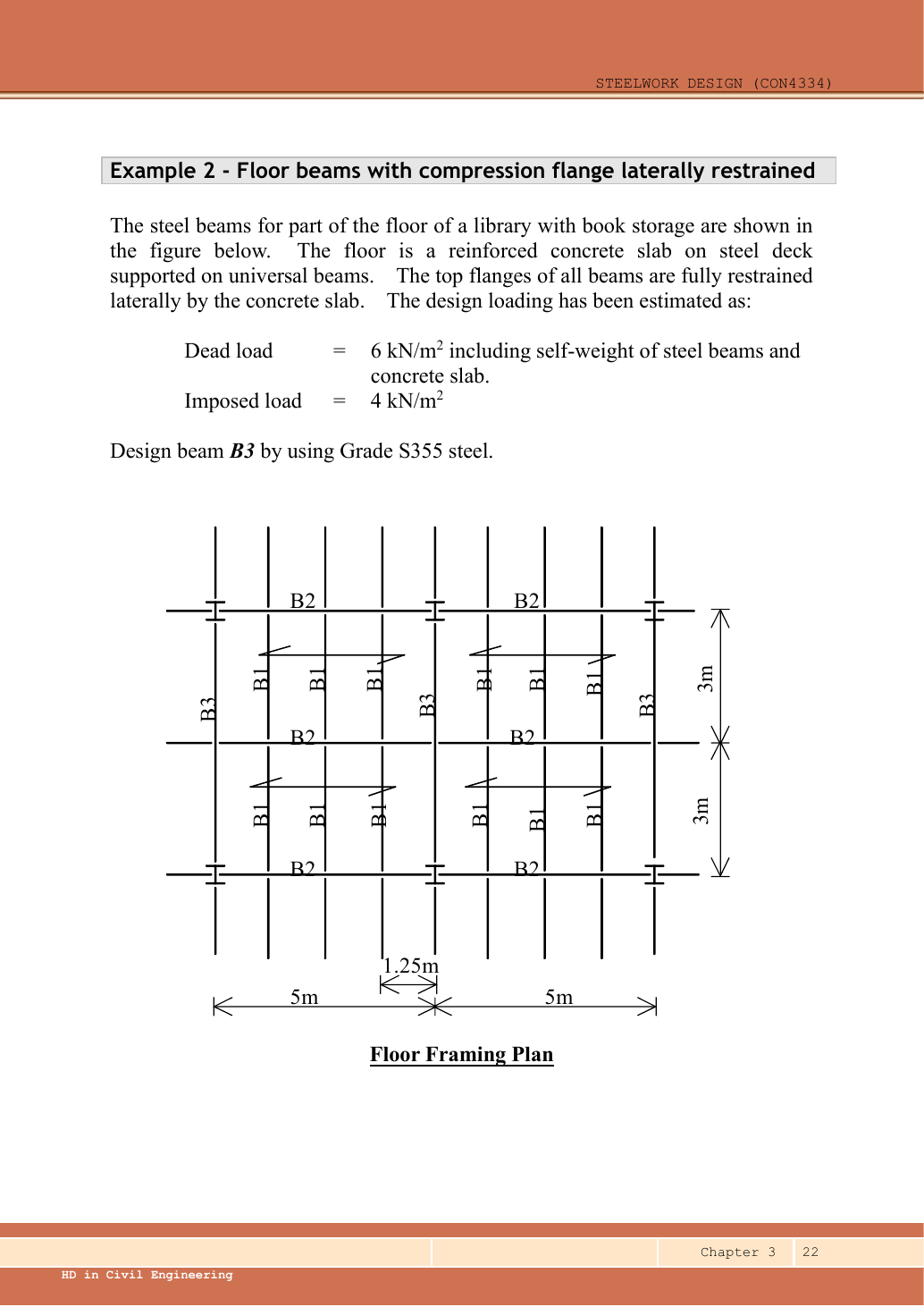
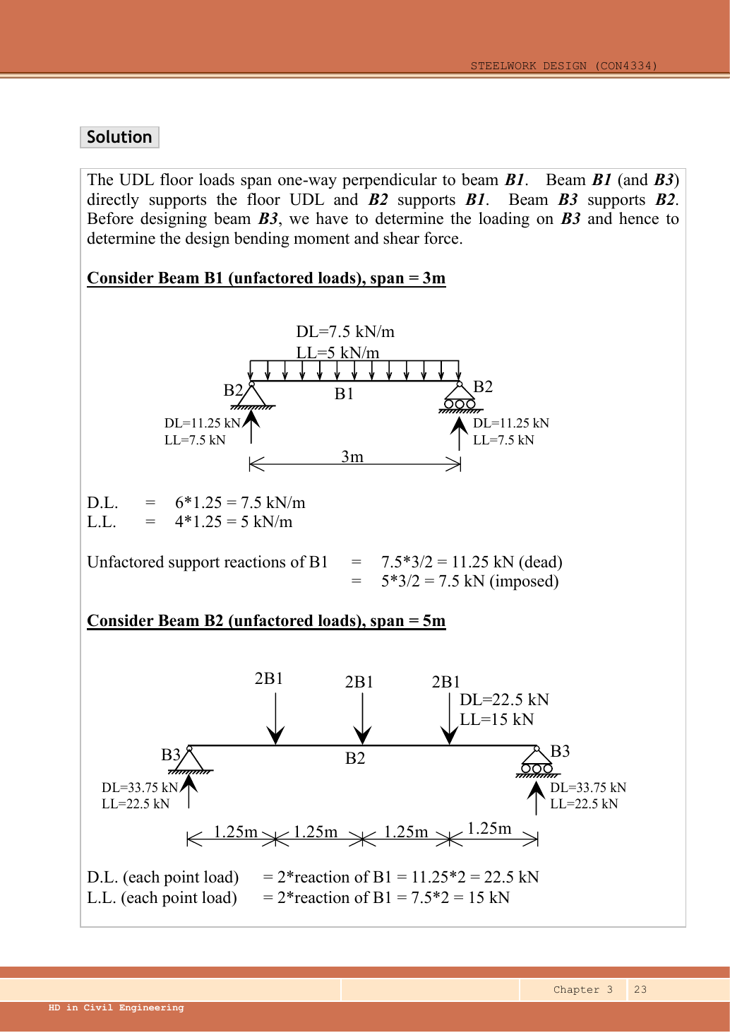
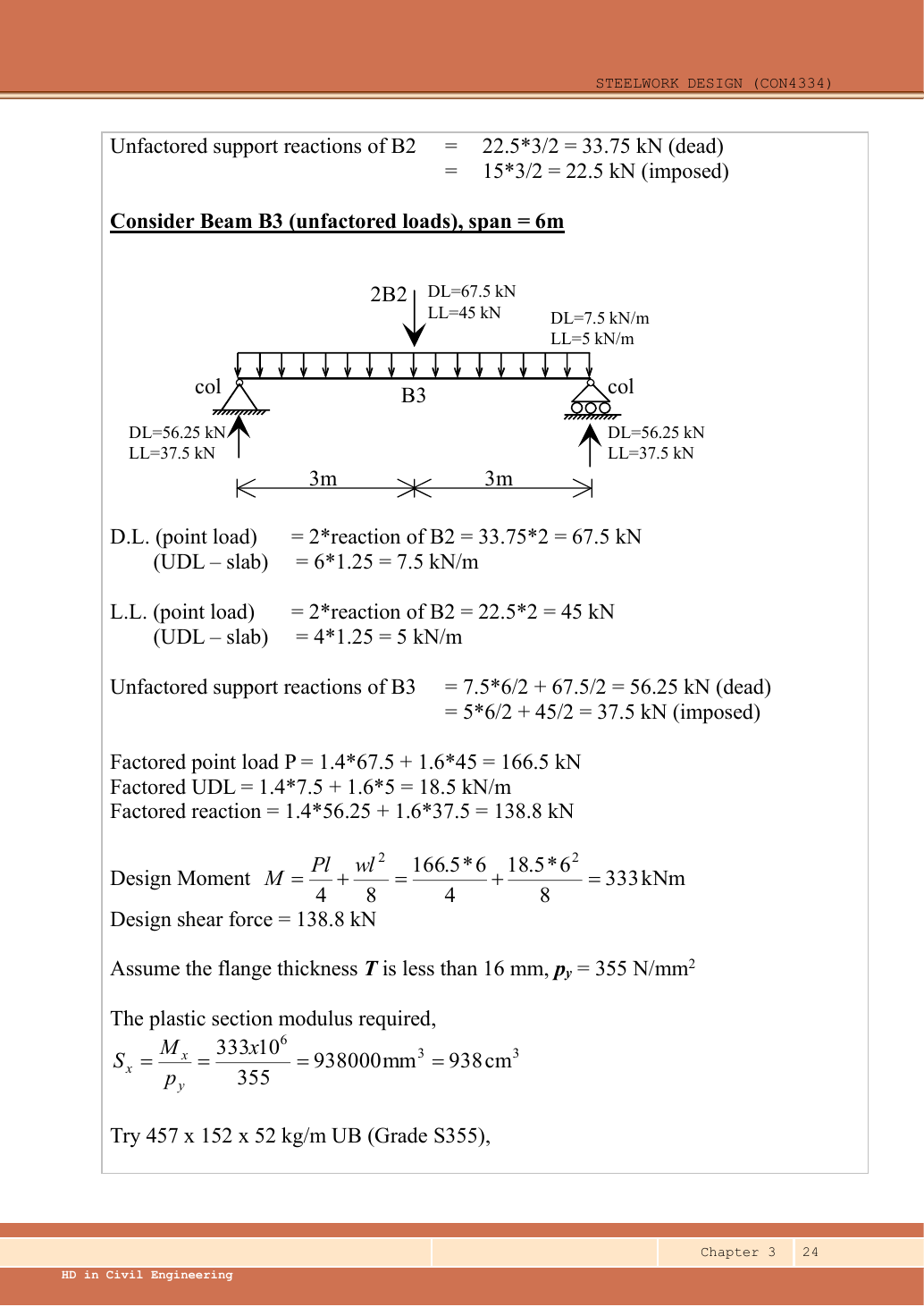
Read the diagram and collect the data
| Feature | Meaning for loading |
|---|---|
| Slab span marks crossing the B1 lines | Slab load reaches the parallel B1 beams over a tributary width. |
| B1 above and below each interior B2 | Each B2 loading point receives two B1 end reactions. |
| B2 on both sides of the interior B3 | B3 receives two B2 end reactions at its centre. |
| B3 also directly borders slab strips | Interior B3 carries its own tributary slab strip, represented as a UDL. |
| Given and assumed | All self-weight is already allowed for in the supplied dead intensity. B3 fully restrained; lecturer assumes brittle finishes for serviceability. |
Before calculating: recognition and strategy
Work upstream before downstream: slab → B1 → B2 → B3. A supporting beam receives a point load equal to the end reaction of the supported beam, not that beam’s entire load. Keep dead and imposed reactions separate until the B3 loading is established. Do not treat the horizontal bay width as the B3 span.
1. Slab to B1
The division by two comes from a uniformly loaded simply supported span. These are characteristic reactions, before the ultimate factors.
Animation labFollow the floor load in 3D
Supplement to the original lesson. Enable JavaScript to play, step through calculations and rotate 3D models. The following explanation remains readable offline.
- The floor carries pressure in . The highlighted strip belongs to one secondary beam.
- Multiply pressure by tributary width: . The illustration uses .
- A primary beam receives the secondary beam reaction at their connection, not a new full-span UDL.
- Trace reactions down to columns and foundations. Count each loaded area once.
2. B1 reactions to B2
There are three internal point loads, not four: four slab strips are bounded by three interior B1 lines and the two B3 boundaries. Symmetry of the three loads gives half the total at each B2 end. Loads arriving directly at column-supported beam ends do not add span bending.
Animation labFollow the floor load in 3D
Supplement to the original lesson. Enable JavaScript to play, step through calculations and rotate 3D models. The following explanation remains readable offline.
- The floor carries pressure in . The highlighted strip belongs to one secondary beam.
- Multiply pressure by tributary width: . The illustration uses .
- A primary beam receives the secondary beam reaction at their connection, not a new full-span UDL.
- Trace reactions down to columns and foundations. Count each loaded area once.
3. Assemble B3 point load and direct slab UDL
Simple explanation: How a floor load reaches a beam
Each beam collects the load from its own strip of floor.
- Find the tributary width from the actual plan.
- Area load × tributary width gives load per beam length.
- A supporting beam receives the other beam’s end reaction.
Remember: A reaction becomes a point load, not automatically a UDL.
The factor of two at the central point represents the B2 on each side of B3. It does not double B3’s span or its tributary strip.
Animation labFollow the floor load in 3D
Supplement to the original lesson. Enable JavaScript to play, step through calculations and rotate 3D models. The following explanation remains readable offline.
- The floor carries pressure in . The highlighted strip belongs to one secondary beam.
- Multiply pressure by tributary width: . The illustration uses .
- A primary beam receives the secondary beam reaction at their connection, not a new full-span UDL.
- Trace reactions down to columns and foundations. Count each loaded area once.
4. Reactions, shear and moment of B3
Simple explanation: Why reactions balance the loads
Think of a seesaw that must neither fall nor turn.
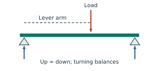
- Upward and downward forces must balance.
- Take moments about a support to eliminate its reaction.
- Use perpendicular distance from the point to the force line.
Remember: A lateral restraint is not automatically a vertical support.
Animation labBalance reactions and moments
Supplement to the original lesson. Enable JavaScript to play, step through calculations and rotate 3D models. The following explanation remains readable offline.
- This demonstrator is a simply supported 6 m beam with a 60 kN point load; it is not the page’s original loading diagram.
- . Moving the load towards B increases .
- . The two upward reactions must sum to P.
- With the load at midspan, . End couples, UDLs and overhangs require their own equilibrium terms.
5. Select UB
Data File p.9 row gives , , , , , and . Page 10, the same designation, gives , , . confirms pᵧ=355. No interpolation is used for section properties: read the exact row.
Animation labRead a table without losing the keys
Supplement to the original lesson. Enable JavaScript to play, step through calculations and rotate 3D models. The following explanation remains readable offline.
- Name the required property: material strength, section property, buckling strength or a moment factor.
- Keep section size, steel grade, thickness band, curve and axis as separate lookup keys.
- , and require different conversion powers. Do not use adjacent columns interchangeably.
- Use bracketing rows within the same valid column. The original page remains the source of all table values.
6. Classify the trial section
Animation labWhy thin elements buckle locally
Supplement to the original lesson. Enable JavaScript to play, step through calculations and rotate 3D models. The following explanation remains readable offline.
- The flange outstand and web have different widths, thicknesses and edge support conditions.
- A thinner plate can wrinkle locally before the complete member loses stability.
- Class 1 allows plastic rotation; Class 2 reaches plastic resistance; Class 3 reaches elastic resistance; Class 4 requires effective properties.
- Check every relevant compression element with the supplied limits and stress distribution. The deformation shown is qualitative.
7. Check shear resistance
Animation labSee shear in the web
Supplement to the original lesson. Enable JavaScript to play, step through calculations and rotate 3D models. The following explanation remains readable offline.
- Internal shear keeps the two sides of the cut in vertical equilibrium.
- For the course’s common I-section case, the web provides the principal shear area; use the specified definition.
- A slender web may require a different shear-buckling route before a simple shear-resistance formula is used.
- Use where applicable in the course. Convert N to kN before comparing with design shear.
8. Check moment resistance
Simple explanation: Why one flange squeezes and the other stretches
Bending makes opposite sides of the section do opposite jobs.
- Find the moment from the actual loads and supports.
- Choose the resistance formula allowed by the section class.
- Check whether the coexistent shear changes that formula.
Remember: Use shear at the location being checked, not an unrelated maximum.
The source’s requested B3 design demonstrates shear, moment and deflection. It does not specify a bearing geometry for a numerical local-web design here. Do not import the bearing from Example 1.
Animation labCompression and tension across a section
Supplement to the original lesson. Enable JavaScript to play, step through calculations and rotate 3D models. The following explanation remains readable offline.
- For sagging, the top flange is in compression and the bottom in tension; hogging reverses this.
- Elastic bending stress varies with distance from the neutral axis: .
- The section class governs whether elastic, plastic or effective properties may be used.
- Use the shear at the section under examination; the largest shear elsewhere is not automatically coexistent.
9. Check B3 serviceability
Simple explanation: How much does the beam sag?
Strength asks whether it fails; deflection asks how far it moves.
- Use the serviceability load case specified by the course question.
- Choose the expression matching the support and load positions.
- Use consistent units for load, length, E and I.
Remember: The largest deflection is not always at midspan.
Animation labSee stiffness and deflection
Supplement to the original lesson. Enable JavaScript to play, step through calculations and rotate 3D models. The following explanation remains readable offline.
- Use the specified SLS load, span and support arrangement. The demonstrator has a full-span UDL.
- The loaded beam bends; the deformation is exaggerated so its shape can be seen.
- For a simply supported full-span UDL, . Double L with w, E and I unchanged: δ becomes 16 times as large.
- The readout uses , and . Select the finish/support-specific limit from the original table.
Compact exam answer
B1 characteristic reactions /=/. B2 has three / points; end reactions /. B3 central /=/ plus /. Ultimate , , , . Select UB S355, Class 1: , , . The demonstrated checks pass.
Mistakes to avoid
- Do not make floor pressure a beam UDL without multiplying by tributary width.
- Do not transfer a supported beam’s entire load to each end.
- Include B3’s directly supported slab strip once.
- Do not add self-weight already included by the problem.
Procedure for an unfamiliar variant
- Identify the vertical supports, span, lateral restraints and individual load positions.
- Keep dead and imposed loads separate; form the required ultimate and serviceability cases.
- Find reactions and the maximum shear/moment by equilibrium, with units.
- Choose a section-table row, confirm thickness-dependent strength, and classify both flange and web.
- Check shear and bending; add segment LTB where restraint is discrete.
- Complete the requested web and deflection checks; state the governing result and any missing data.
Independent self-check
Try it yourself. Invented variant: only the characteristic floor imposed pressure rises from to . Find the revised B3 ultimate and , and imposed deflection; retain the original dead loading.
Reveal answer and reasoning
All imposed effects multiply by . B3 imposed point; imposed UDL. ; . . Imposed deflection=. Maximum shear=; these checks still pass.
Animation labFollow the floor load in 3D
Supplement to the original lesson. Enable JavaScript to play, step through calculations and rotate 3D models. The following explanation remains readable offline.
- The floor carries pressure in . The highlighted strip belongs to one secondary beam.
- Multiply pressure by tributary width: . The illustration uses .
- A primary beam receives the secondary beam reaction at their connection, not a new full-span UDL.
- Trace reactions down to columns and foundations. Count each loaded area once.
Animation labFollow the calculation sequence
Supplement to the original lesson. Enable JavaScript to play, step through calculations and rotate 3D models. The following explanation remains readable offline.
- Locate the load, supports, connection geometry and any stated assumptions.
- Keep given values, table lookups and calculated values distinct; reconcile their units.
- The calculation player steps through the existing expressions in their original order.
- Compare demand with resistance or the relevant limit. Keep missing inputs and conditional conclusions explicit.
8. Normal versus destabilizing loads Background
The lecture’s definition: the main loads act on the top flange, and both the load and the flange are free to move and rotate relative to the shear centre. An arrow drawn on top of the beam is not enough to decide this. If the question says “normal load”, treat it as normal — exam questions usually are.
Animation labA beam bends sideways and twists
Supplement to the original lesson. Enable JavaScript to play, step through calculations and rotate 3D models. The following explanation remains readable offline.
- For the illustrated sagging beam the top flange is compressed.
- The unrestrained compression flange can move sideways while the complete cross-section twists.
- Only effective restraints divide the member into unbraced segments. They do not automatically add vertical supports.
- Use the segment effective length, section properties and matching moment factor. This is an exaggerated mode shape, not a calculated displacement.
9. LTB effective length Always examined
Simple explanation: Which length belongs in the calculation?
A sideways tie can shorten the buckling region without shortening the beam’s vertical span.
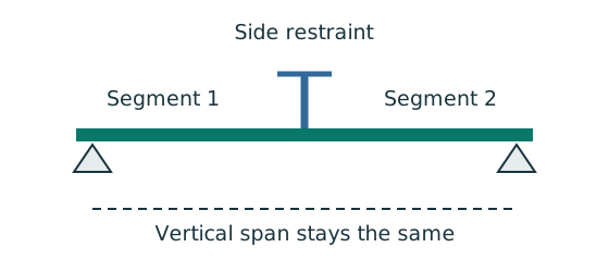
- Separate vertical-support spacing from lateral-restraint spacing.
- Apply the course rule for the actual end restraint and loading.
- Keep the original vertical load analysis unless its supports change.
Remember: Restraints in one direction may not restrain the other direction.
| Source condition, Ch 3 p.9 | Effective length for normal load |
|---|---|
| End compression-flange lateral restraint, free rotation in plan, nominal torsional restraint | |
| Compression flange fully restrained against rotation in plan at end supports | |
| End compression flanges not laterally restrained; both flanges free to rotate in plan | |
| Adequate intermediate lateral restraints | Lᴇ=segment length Lᴸᵀ |
For destabilizing loads multiply the length by 1.2 (intermediate segments use ). If the question says the effective length equals the segment length, follow it. Cantilever segments cannot use the table above; use Table 8.1 (below).
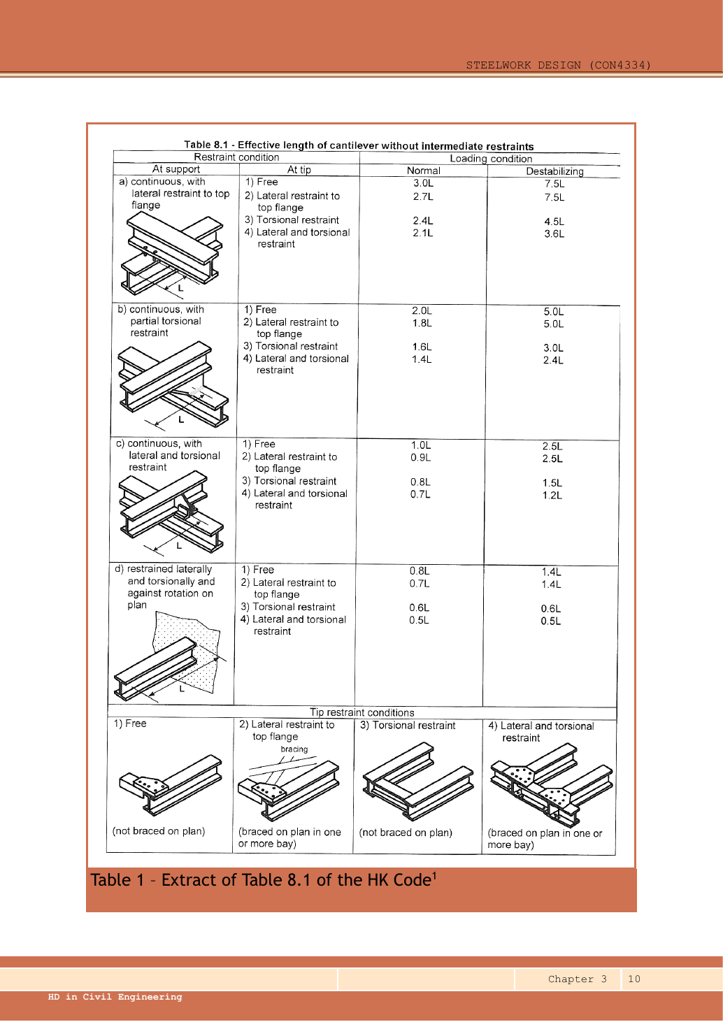
(a1) /; (a2) /; (a3) /; (a4) /.
(b1) /; (b2) /; (b3) /; (b4) /.
(c1) /; (c2) /; (c3) /; (c4) /.
(d1) /; (d2) /; (d3) /; (d4) /. Open full-size image
To read Table 8.1: choose the support group (a–d), then the tip row (1–4), then the normal / destabilizing column. For example group (c), free tip (1), normal load → ; the same case with a destabilizing load → .
Animation labA beam bends sideways and twists
Supplement to the original lesson. Enable JavaScript to play, step through calculations and rotate 3D models. The following explanation remains readable offline.
- For the illustrated sagging beam the top flange is compressed.
- The unrestrained compression flange can move sideways while the complete cross-section twists.
- Only effective restraints divide the member into unbraced segments. They do not automatically add vertical supports.
- Use the segment effective length, section properties and matching moment factor. This is an exaggerated mode shape, not a calculated displacement.
10. From length to : the LTB look-up routine Always examined
Simple explanation: A beam can escape sideways
The compressed flange can move sideways while the section twists.
- Divide the beam at effective lateral restraints.
- Use each segment’s effective length to obtain its buckling resistance.
- Compare that resistance with the segment’s equivalent moment demand.
Remember: A section bending check alone does not check lateral-torsional buckling.
is the minor-axis radius of gyration; its units must match (the table gives cm, so ×10 for mm). (buckling parameter) and (torsional index) come from the same table row — this is not a position. For Class 1 and 2 sections . The lecture allows and for a rough first check, but exam questions usually ask for the accurate values.
In Table 8.3a choose the right column: S355 with a 20 mm flange → the 345 column, not 355. Find the two rows either side of and interpolate. Never look up directly.
Try it yourself. λᴸᵀ=121.6 and pᵧ=355. Rows and give and . Find pᵦ.
Reveal answer and reasoning
Interpolation fraction . , conventionally written .
Animation labA beam bends sideways and twists
Supplement to the original lesson. Enable JavaScript to play, step through calculations and rotate 3D models. The following explanation remains readable offline.
- For the illustrated sagging beam the top flange is compressed.
- The unrestrained compression flange can move sideways while the complete cross-section twists.
- Only effective restraints divide the member into unbraced segments. They do not automatically add vertical supports.
- Use the segment effective length, section properties and matching moment factor. This is an exaggerated mode shape, not a calculated displacement.
Animation labA beam bends sideways and twists
Supplement to the original lesson. Enable JavaScript to play, step through calculations and rotate 3D models. The following explanation remains readable offline.
- For the illustrated sagging beam the top flange is compressed.
- The unrestrained compression flange can move sideways while the complete cross-section twists.
- Only effective restraints divide the member into unbraced segments. They do not automatically add vertical supports.
- Use the segment effective length, section properties and matching moment factor. This is an exaggerated mode shape, not a calculated displacement.
11. Equivalent moment factor : the shape of the moment diagram Always examined
Simple explanation: Why the shape of the moment diagram matters
The same peak moment is more demanding when a long region stays near that peak.
- Use the diagram of this unrestrained segment.
- Choose the applicable course sketch or quarter-point rule.
- Apply its factor to the demand, following the stated check.
Remember: Column flexural-buckling factors and LTB factors are not interchangeable.
Use Table 8.4a only when the real moment diagram matches its sketch. For a straight-line diagram (end moments, no load in between): = smaller end moment ÷ larger end moment (positive if both are on the same side, negative if the diagram crosses zero), .
In the quarter-point formula take all moments as positive (magnitudes), even if the diagram crosses zero. The quarter points are ¼, ½ and ¾ of this segment, not of the whole beam; work out those moments by equilibrium, including any UDL. A cantilever segment without intermediate restraint uses .
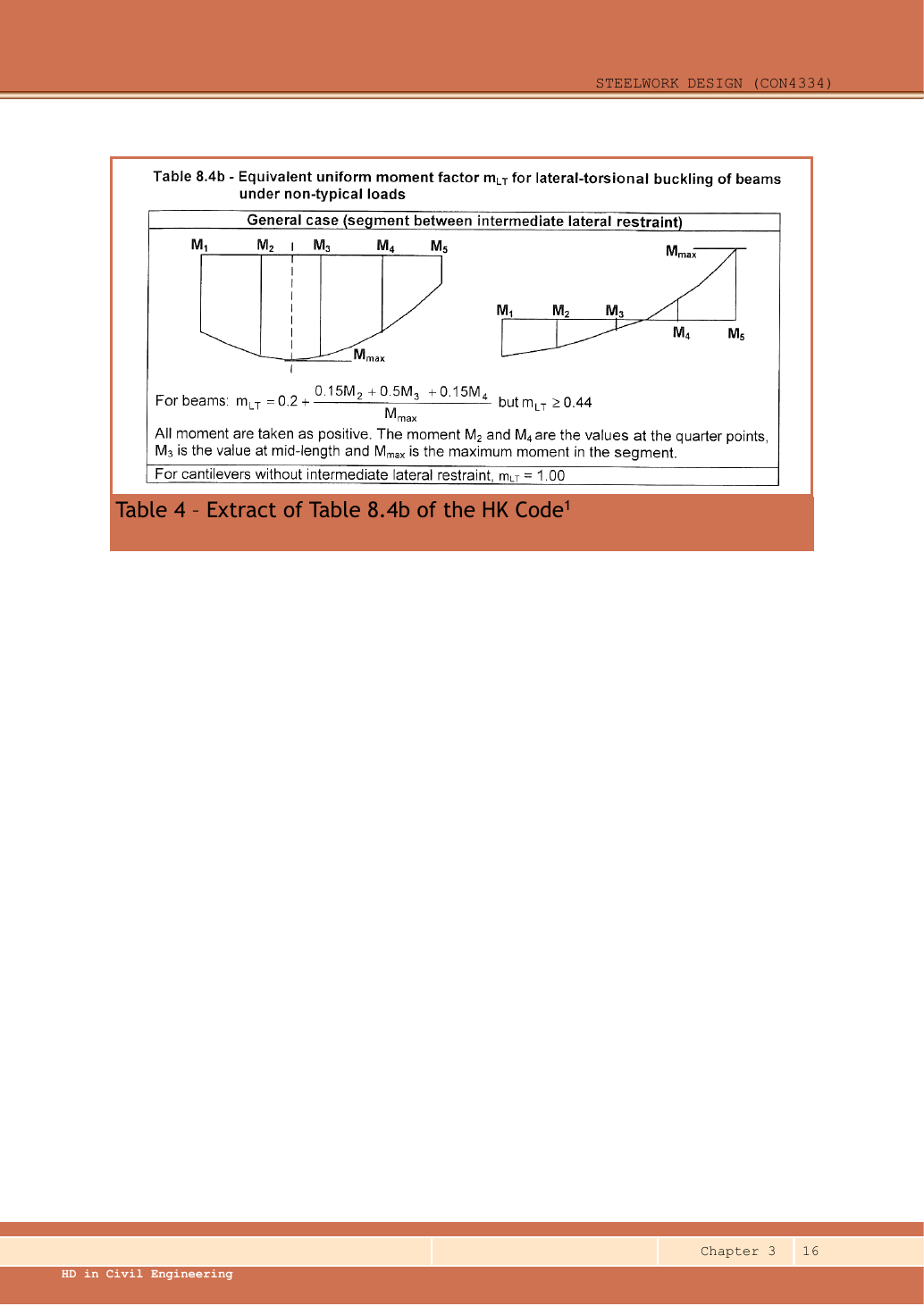
Animation labRead the moment shape within one segment
Supplement to the original lesson. Enable JavaScript to play, step through calculations and rotate 3D models. The following explanation remains readable offline.
- Moment ordinates must belong to the same effective unbraced segment.
- Same-side and reverse-curvature diagrams have different signed end ratios.
- The markers show ¼, ½ and ¾ of this segment, not of the entire beam.
- LTB and column flexural factors are different. Preserve their individual bounds and coefficient sets.
12. Full LTB procedure (Section B) Always examined
- Find the reactions, SFD and BMD of the whole beam using the real vertical supports.
- Mark every lateral restraint and divide the beam into segments.
- For each segment work out and .
- Find each segment’s maximum moment and ; check .
- Separately check the section: and (high shear if needed).
- Do any web and deflection checks asked for, and say which segment governs.
The segment with the biggest moment is not always the critical one: a longer, less restrained segment may have a much smaller . List the demand, resistance and ratio for every segment in a small table.
Understanding map: LTB check: where every number comes from and where it goes
Understanding map
LTB check: where every number comes from and where it goes
The hardest part of the LTB question is knowing which number goes into which formula. Read the map from top to bottom in answer order: numbers from the question and the tables at the top, the conclusion at the bottom. The values are from 2024 BQ4, segment BC (4 m).
- From the question
- From the tables
- Worked out
- Demand
- Capacity
- Check
- marks are often lost here
Text version (in working order)
From the questionWhere marks are lost
Segment length
Lateral restraints split the beam into segments, each checked on its own. Segment BC runs from B (3.5 m) to C (7.5 m).
Needs (upstream)— (a starting value)
Used for (downstream), , Quarter-point moments Largest moment in segment Effective length
From the questionWhere marks are lost
, Loads and supports
The design loads (already factored) and where the supports are. Only points drawn with a support symbol have reactions.
2024 BQ4 (segment BC)
Needs (upstream)— (a starting value)
Used for (downstream), Support reactions
From the tablesWhere marks are lost
Minor-axis radius of gyration
How “stocky” the section is about its weak axis. The larger it is, the harder it is to bow sideways.
Where it comes from: Section table (5.03 cm → 50.3 mm).
Needs (upstream)— (a starting value)
Used for (downstream) Slenderness
Worked out
Effective length
Normal load with restraints at both ends → segment length. Load on the top flange that can move sideways with it (destabilizing) → ×1.2. Cantilevers: Table 8.1.
Formula
2024 BQ4 (segment BC)
Needs (upstream) Segment length
Used for (downstream) Slenderness
Worked out
, Support reactions
Take moments about one support to find the other reaction; the two must add up to the total load.
Formula
2024 BQ4 (segment BC)
Needs (upstream), Loads and supports
Used for (downstream) Bending-moment diagram
From the tablesWhere marks are lost
Design strength
Look it up from the grade and the flange thickness . S355 with a flange thicker than 16 mm gives 345.
2024 BQ4 (segment BC)
Where it comes from: Data File design-strength table; from the section table. Core skills §5
Needs (upstream)— (a starting value)
Used for (downstream) Section factor Bending strength
From the tablesWhere marks are lost
Torsional index
A measure of how the section resists twisting; used only in the formula.
Where it comes from: Same section-table row.
Needs (upstream)— (a starting value)
Used for (downstream) Slenderness factor
Worked outWhere marks are lost
Slenderness
Length compared with stockiness. The larger it is, the more slender the segment and the easier it buckles.
Formula
2024 BQ4 (segment BC)
Needs (upstream) Effective length Minor-axis radius of gyration
Used for (downstream) Slenderness factor Equivalent slenderness
Worked out
Bending-moment diagram
Work out the shear and moment point by point from the reactions. Where the shear changes from positive to negative is the maximum moment.
Formula
2024 BQ4 (segment BC)
Where it comes from: Method: core skills §3.
Needs (upstream), Support reactions
Used for (downstream), , Quarter-point moments Largest moment in segment
Worked out
Section factor
Class 1 or 2 section → . Classification uses , which comes from .
Where it comes from: Section classification (core skills §6).
Needs (upstream) Design strength
Used for (downstream) Equivalent slenderness
From the tables
Buckling parameter
A section-shape factor, read straight from the table.
Where it comes from: Same section-table row.
Needs (upstream)— (a starting value)
Used for (downstream) Equivalent slenderness
Worked out
Slenderness factor
A correction for twisting of the section, set by ; always below 1.
Formula
2024 BQ4 (segment BC)
Needs (upstream) Slenderness Torsional index
Used for (downstream) Equivalent slenderness
Worked outWhere marks are lost
, , Quarter-point moments
The moments at ¼, ½ and ¾ of this segment. For BC that is 1, 2 and 3 m from B, i.e. 4.5, 5.5 and 6.5 m from A.
2024 BQ4 (segment BC)
Needs (upstream) Bending-moment diagram Segment length
Used for (downstream) Equivalent moment factor
Demand
Largest moment in segment
The largest moment (ignoring sign) inside this segment. For BC it is at C.
Needs (upstream) Bending-moment diagram Segment length
Used for (downstream) Equivalent moment factor Equivalent moment (demand)
Worked out
Equivalent slenderness
Slenderness that also accounts for the section shape (). This is the number used to look up .
Formula
2024 BQ4 (segment BC)
Needs (upstream) Buckling parameter Slenderness factor Slenderness Section factor
Used for (downstream) Bending strength
Worked out
Equivalent moment factor
Turns an uneven moment into an equivalent uniform one. Close to the peak all along → near 1; peak at one point only → smaller, but never below 0.44.
Formula
2024 BQ4 (segment BC)
Needs (upstream), , Quarter-point moments Largest moment in segment
Used for (downstream) Equivalent moment (demand)
From the tables
Plastic modulus
The modulus of the fully yielded section (cm³); it turns the strength into a moment.
Where it comes from: Section table, the 610×229×140 UB row.
Needs (upstream)— (a starting value)
Used for (downstream) Buckling resistance moment
Worked outWhere marks are lost
Bending strength
Interpolate in Table 8.3a, in the column, using . The larger (more slender), the smaller .
Formula
2024 BQ4 (segment BC)
Where it comes from: Data File p.5, Table 8.3a, column.
Needs (upstream) Equivalent slenderness Design strength
Used for (downstream) Buckling resistance moment
Demand
Equivalent moment (demand)
The moment this segment really has to carry; it is compared with at the end.
2024 BQ4 (segment BC)
Needs (upstream) Equivalent moment factor Largest moment in segment
Used for (downstream) Segment BC conclusion
Capacity
Buckling resistance moment
The largest moment this segment can carry before it buckles sideways.
Formula
2024 BQ4 (segment BC)
Needs (upstream) Bending strength Plastic modulus
Used for (downstream) Segment BC conclusion
Check
Segment BC conclusion
If the demand is not larger than the capacity, the segment passes. Write this conclusion for every segment.
2024 BQ4 (segment BC)
Needs (upstream) Equivalent moment (demand) Buckling resistance moment
Used for (downstream)— (the final conclusion)
Tour steps
1. Find the segment
Read the drawing: supports give reactions; restraint crosses (×) split the beam into segments. BC is 4 m long, and everything below is worked out for this segment only.
In this step, Loads and supports Segment length
2. Reactions and moment diagram (7 marks)
The same skill as the compulsory floor beams: take moments for the reactions, then work out shear and moment at each point and label them.
In this step, Support reactions Bending-moment diagram
3. The demand on this segment
Take the quarter-point moments and the maximum inside the segment, work out , then multiply by to get the demand, 558.1 kN·m.
In this step, , Quarter-point moments Largest moment in segment Equivalent moment factor Equivalent moment (demand)
4. One trip to the tables
Copy from the same section-table row; from ; Class 1 → .
In this step Design strength Section factor Plastic modulus Minor-axis radius of gyration Buckling parameter Torsional index
5. From length to slenderness
comes from the segment length; ; comes from .
In this step Effective length Slenderness Slenderness factor
6. Equivalent slenderness
— four arrows meet here, and this is the number for the table.
In this step Equivalent slenderness
7. Look up , work out
Interpolate in the 345 column of Table 8.3a, then multiply by to get the capacity .
In this step Bending strength Buckling resistance moment
8. Compare and conclude
558.1 < 973.4 → segment BC passes. Walk the same path again for CD (2024 answer: 365.8 < 1075.1 ✓).
In this step Segment BC conclusion
Beam example 3: three restrained segments and an omitted deflection solution
Open this example on its own page
Check/design the S355 simply supported beam for shear and bending with lateral restraints at A, B, C and D. . At B: dead and imposed ; at C: dead and imposed . Dead self-weight is . Effective segment lengths equal actual lengths. Also work through the lecturer’s requested follow-up web and deflection checks.
Original source: LectureNotes/Ch 3_Beam.pdf — p. 27, p. 28, p. 29, p. 30. Values tagged given are in the question or diagram; lookup values come from a named table; calculated values follow from the working; assumptions are stated explicitly.
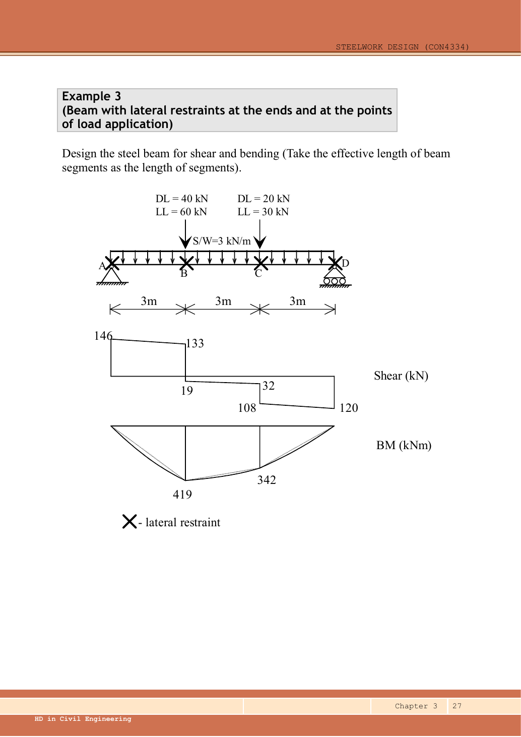
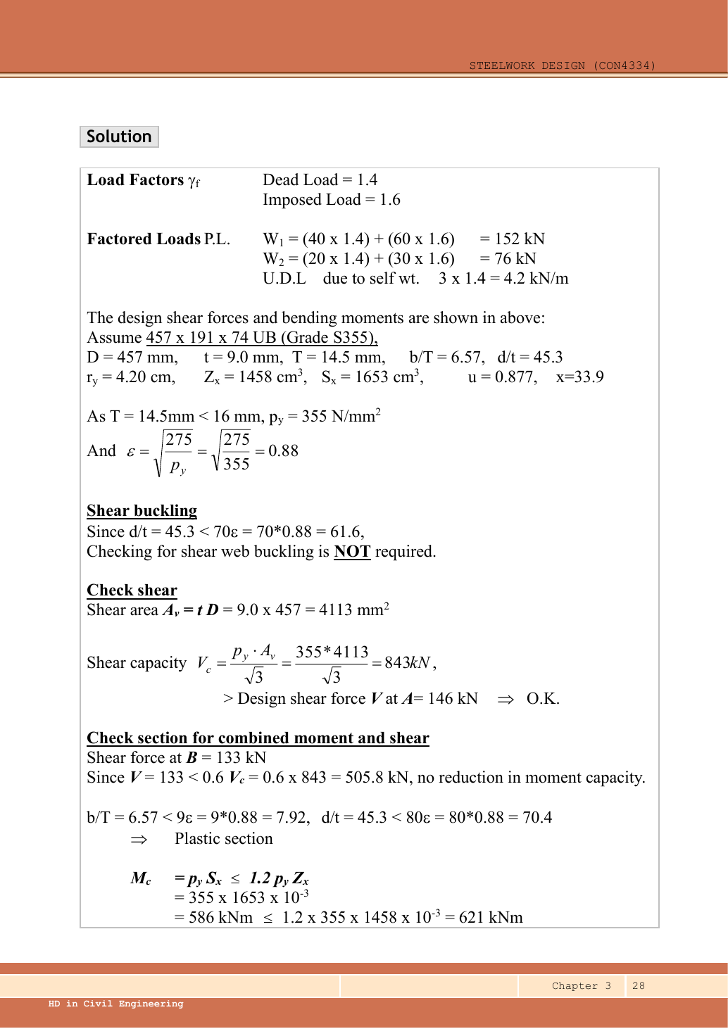
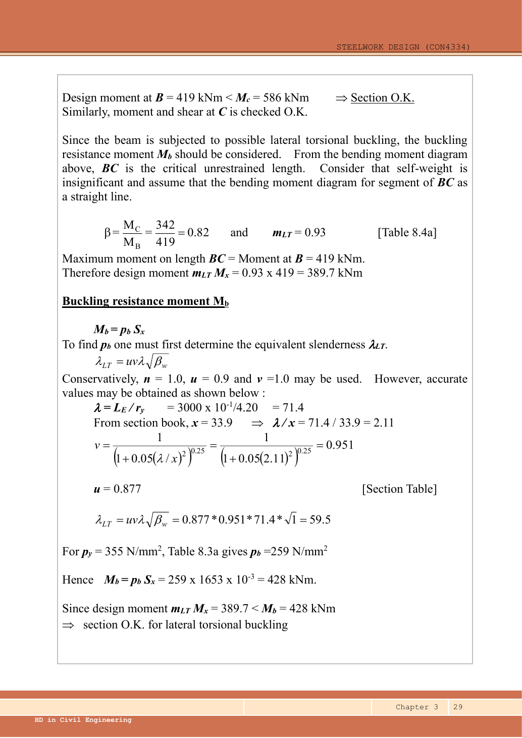
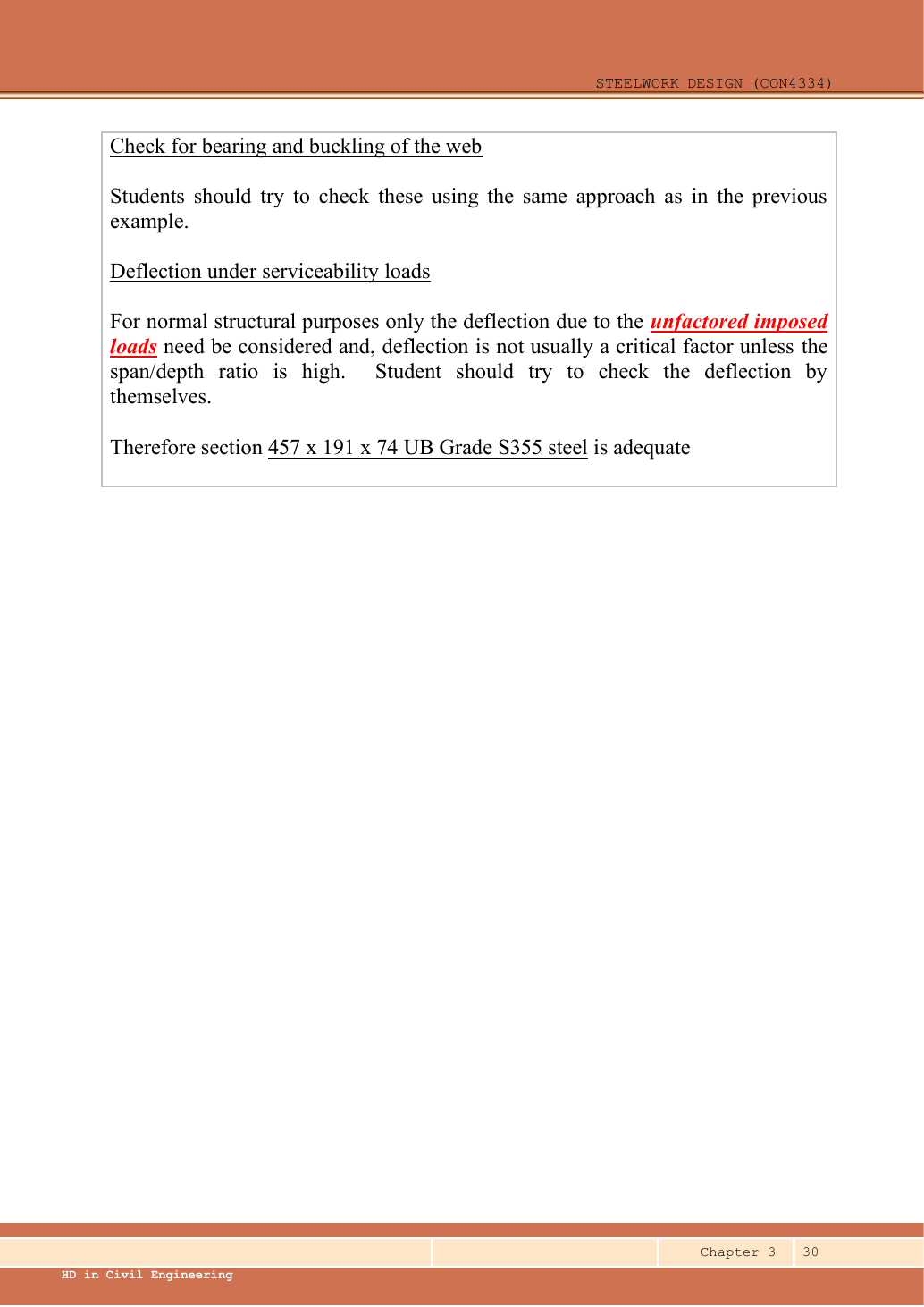
Read the diagram and collect the data
| Input | Exact diagram or table source |
|---|---|
| Vertical span | Three dimension strings of give . |
| Lateral model | Crosses define three unbraced segments; question sets Lᴇ=3,000 mm. |
| Trial section | The source selects UB. Data pp.9–10 give , , , , ; , ; ; ; , ; , . |
| Missing local-web data | No stiff bearing lengths, distances to member ends or complete local flange-restraint details are given. Crosses alone identify lateral restraint, not both web-buckling conditions. |
Before calculating: recognition and strategy
Analyse the continuous beam on its two vertical supports. Use that BMD to examine the three separate lateral-buckling segments. First reproduce the lecturer’s rounded, straight-line BC approximation, then retain the self-weight curvature with Table 8.4b to check every segment. Deflection uses the imposed loads and at their actual off-centre positions; a central-point formula cannot be substituted.
1. Factored loads
Animation labFrom characteristic to design load
Supplement to the original lesson. Enable JavaScript to play, step through calculations and rotate 3D models. The following explanation remains readable offline.
- G is permanent load; Q is imposed load. A surface load and a line load also have different units.
- This illustration uses the course gravity case . Other combinations in the original text retain their own factors.
- For illustrative , change Q and watch each separate contribution.
- Do not carry this ULS total automatically into deflection. Follow the stated SLS load case.
2. Reactions without premature rounding
Simple explanation: Why reactions balance the loads
Think of a seesaw that must neither fall nor turn.
- Upward and downward forces must balance.
- Take moments about a support to eliminate its reaction.
- Use perpendicular distance from the point to the force line.
Remember: A lateral restraint is not automatically a vertical support.
Take moments about D: each downward load contributes its distance to D; the UDL resultant acts at midspan, from D.
Check by moments about A:.
Animation labBalance reactions and moments
Supplement to the original lesson. Enable JavaScript to play, step through calculations and rotate 3D models. The following explanation remains readable offline.
- This demonstrator is a simply supported 6 m beam with a 60 kN point load; it is not the page’s original loading diagram.
- . Moving the load towards B increases .
- . The two upward reactions must sum to P.
- With the load at midspan, . End couples, UDLs and overhangs require their own equilibrium terms.
3. Construct the SFD and BMD from the left-hand free body
For moment (), start with ; when , add ; when , also add . Each negative term is a point load times its lever arm to the section; include it only after the section has passed that load.
Read each “when” term as zero before its load position and include it afterwards. is in metres from A. The shorthand is often written with positive-part brackets ; it is a beam-position coordinate, unrelated to the torsional index.
| Position | Shear just left / right () | Moment () |
|---|---|---|
| / | ||
| B, | / | |
| C, | / | |
| / |
B is the maximum because shear changes from positive to negative there. BC and CD have negative shear throughout, so their bending moment decreases. Draw straight sloping shear segments, vertical jumps at the point loads, and curved bending segments continuous at B and C.
Animation labBuild the shear and moment diagrams
Supplement to the original lesson. Enable JavaScript to play, step through calculations and rotate 3D models. The following explanation remains readable offline.
- For the illustrative 60 kN point load on a 6 m simply supported beam, balance the reactions before making a cut.
- and before the point load. Moment grows linearly.
- Shear jumps down by P. To its right, and .
- For this case, moment is continuous and returns to zero at B. A concentrated applied couple instead creates a moment jump.
4. Confirm strength and section class
Animation labWhy thin elements buckle locally
Supplement to the original lesson. Enable JavaScript to play, step through calculations and rotate 3D models. The following explanation remains readable offline.
- The flange outstand and web have different widths, thicknesses and edge support conditions.
- A thinner plate can wrinkle locally before the complete member loses stability.
- Class 1 allows plastic rotation; Class 2 reaches plastic resistance; Class 3 reaches elastic resistance; Class 4 requires effective properties.
- Check every relevant compression element with the supplied limits and stress distribution. The deformation shown is qualitative.
5. Shear resistance
Animation labSee shear in the web
Supplement to the original lesson. Enable JavaScript to play, step through calculations and rotate 3D models. The following explanation remains readable offline.
- Internal shear keeps the two sides of the cut in vertical equilibrium.
- For the course’s common I-section case, the web provides the principal shear area; use the specified definition.
- A slender web may require a different shear-buckling route before a simple shear-resistance formula is used.
- Use where applicable in the course. Convert N to kN before comparing with design shear.
6. Actual section moment resistance
Animation labCompression and tension across a section
Supplement to the original lesson. Enable JavaScript to play, step through calculations and rotate 3D models. The following explanation remains readable offline.
- For sagging, the top flange is in compression and the bottom in tension; hogging reverses this.
- Elastic bending stress varies with distance from the neutral axis: .
- The section class governs whether elastic, plastic or effective properties may be used.
- Use the shear at the section under examination; the largest shear elsewhere is not automatically coexistent.
7. Check every unbraced segment
Simple explanation: A beam can escape sideways
The compressed flange can move sideways while the section twists.
- Divide the beam at effective lateral restraints.
- Use each segment’s effective length to obtain its buckling resistance.
- Compare that resistance with the segment’s equivalent moment demand.
Remember: A section bending check alone does not check lateral-torsional buckling.
All three segments have the same section and effective length, hence the same buckling resistance. Use the weak-axis radius .
Lecturer route: approximate BC as straight, ; read mᴸᵀ≈0.93, giving . Rounded λᴸᵀ≈59.5 gives pᵦ≈259 and Mᵦ≈428 kNm. It passes. To include the UDL exactly, use quarter-point magnitudes from above:
| Segment | Quarter positions from A () | 、、() | () | () |
|---|---|---|---|---|
For AB insert its three ordinates into the same expression:. For CD:. Their factors also exceed . BC governs and all three pass.
Animation labA beam bends sideways and twists
Supplement to the original lesson. Enable JavaScript to play, step through calculations and rotate 3D models. The following explanation remains readable offline.
- For the illustrated sagging beam the top flange is compressed.
- The unrestrained compression flange can move sideways while the complete cross-section twists.
- Only effective restraints divide the member into unbraced segments. They do not automatically add vertical supports.
- Use the segment effective length, section properties and matching moment factor. This is an exaggerated mode shape, not a calculated displacement.
8. The omitted local web checks: what can and cannot be concluded
Simple explanation: A concentrated force can hurt one small region
A narrow contact presses much harder locally than the same force spread over a wider contact.
- Find the actual stiff bearing length and end position.
- Check local crushing and local web buckling separately.
- Use the restraint conditions required by each expression.
Remember: Missing contact dimensions cannot be guessed from drawing scale.
Page 30 asks students to check bearing and web buckling, but neither the support bearing geometry nor the load-introduction details at B and C are supplied. A lateral-restraint cross does not specify the stiff bearing length or rotational restraint of the loaded flange relative to the web. Therefore the numerical local-web follow-up remains incomplete from the available source data.
Once ,, and both local restraint conditions are known, evaluate using and the correct end/interior branch in the web-buckling procedure. If local restraint is absent, Lᴱ,web is also needed. Do not copy Example 1’s , and values into this different diagram. The source’s overall “adequate” statement is supported for shear, section bending and LTB, but local-web adequacy is not established by the supplied information.
Animation labSpread a concentrated force into the web
Supplement to the original lesson. Enable JavaScript to play, step through calculations and rotate 3D models. The following explanation remains readable offline.
- A concentrated reaction first enters through the bearing/contact region.
- The flange and root geometry spread the force before it enters the web.
- A wider effective bearing region can reduce local stress for the same force.
- End distance, stiff bearing length and restraint conditions must come from the original question. This slider is illustrative only.
9. Complete the omitted off-centre deflection calculation
Simple explanation: How much does the beam sag?
Strength asks whether it fails; deflection asks how far it moves.
- Use the serviceability load case specified by the course question.
- Choose the expression matching the support and load positions.
- Use consistent units for load, length, E and I.
Remember: The largest deflection is not always at midspan.
Use only the locations and their imposed loads , and of ; there is no imposed UDL. This calculation uses , , constant , and exact section-table value . Imposed-load reactions are , .
The general method starts from the curvature relationship. Taking downward deflection as positive, . Integrate the bending moment twice. Define as follows: when , its value is zero; when , its value is . Use the support conditions to determine the integration constants.
Maximum downward deflection occurs where slope . It lies between B and C: slope numerator at is; at it is, and the positive bending moment makes slope decrease continuously.
At midspan the deflection is , close but not the exact maximum. The source does not specify the finish category for this example. If the brittle-finish criterion used in preceding examples is adopted explicitly, the limit is and passes. The calculated deflection is determined; the acceptance statement is conditional on that chosen serviceability limit.
Animation labSee stiffness and deflection
Supplement to the original lesson. Enable JavaScript to play, step through calculations and rotate 3D models. The following explanation remains readable offline.
- Use the specified SLS load, span and support arrangement. The demonstrator has a full-span UDL.
- The loaded beam bends; the deformation is exaggerated so its shape can be seen.
- For a simply supported full-span UDL, . Double L with w, E and I unchanged: δ becomes 16 times as large.
- The readout uses , and . Select the finish/support-specific limit from the original table.
Compact exam answer
UB S355 is Class 1. Rₐ/Rᴅ=/; Mᴮ/Mᶜ=/. ; . All segments Lᴱ=3 m: λᴸᵀ=59.5807,pᵦ=258.426,Mᵦ=427.178 kNm. Exact equivalent demands AB/BC/CD//; all pass, BC controls. Imposed at ; passes if applies. Local bearing/web-buckling numerical checks are unresolved because bearing and local-restraint data are missing.
Mistakes to avoid
- Do not turn B and C into vertical supports.
- Do not use as the span for the whole-beam deflection.
- Do not omit BC end moments when evaluating its quarter points.
- Do not present assumed bearing dimensions as given.
Procedure for an unfamiliar variant
- Identify the vertical supports, span, lateral restraints and individual load positions.
- Keep dead and imposed loads separate; form the required ultimate and serviceability cases.
- Find reactions and the maximum shear/moment by equilibrium, with units.
- Choose a section-table row, confirm thickness-dependent strength, and classify both flange and web.
- Check shear and bending; add segment LTB where restraint is discrete.
- Complete the requested web and deflection checks; state the governing result and any missing data.
Independent self-check
Try it yourself. Invented variant: with all loads unchanged, the lateral restraint at C is removed. Which parts of this solution must be recalculated?
Reveal answer and reasoning
Vertical reactions, whole-beam SFD/BMD, section shear/bending and elastic deflection do not change. LTB segments become and . For BD use Lᴱ=6,000 mm (if the same effective-length rule is stipulated), recompute ,,λᴸᵀ,pᵦ and Mᵦ, and use quarter positions with the true BD maximum atB. The point load atC remains even though its lateral restraint is removed.
Animation labSee stiffness and deflection
Supplement to the original lesson. Enable JavaScript to play, step through calculations and rotate 3D models. The following explanation remains readable offline.
- Use the specified SLS load, span and support arrangement. The demonstrator has a full-span UDL.
- The loaded beam bends; the deformation is exaggerated so its shape can be seen.
- For a simply supported full-span UDL, . Double L with w, E and I unchanged: δ becomes 16 times as large.
- The readout uses , and . Select the finish/support-specific limit from the original table.
Beam example 4: a tight LTB check with three point loads
Open this example on its own page
Select/check a S355 simply supported beam of span carrying three characteristic point loads, each dead plus imposed, and a dead UDL. Loading is normal. Ends are restrained against torsion, with compression flange free to rotate in plan; there is no intermediate lateral restraint.
Original source: LectureNotes/Ch 3_Beam.pdf — p. 31, p. 32, p. 33. Values tagged given are in the question or diagram; lookup values come from a named table; calculated values follow from the working; assumptions are stated explicitly.
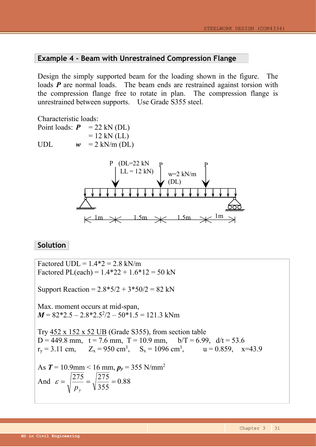
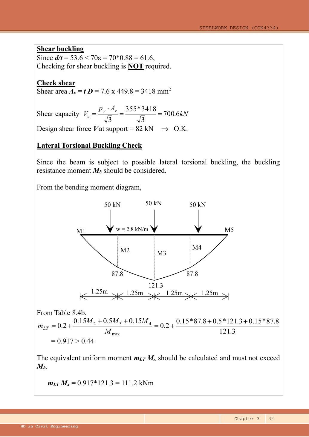
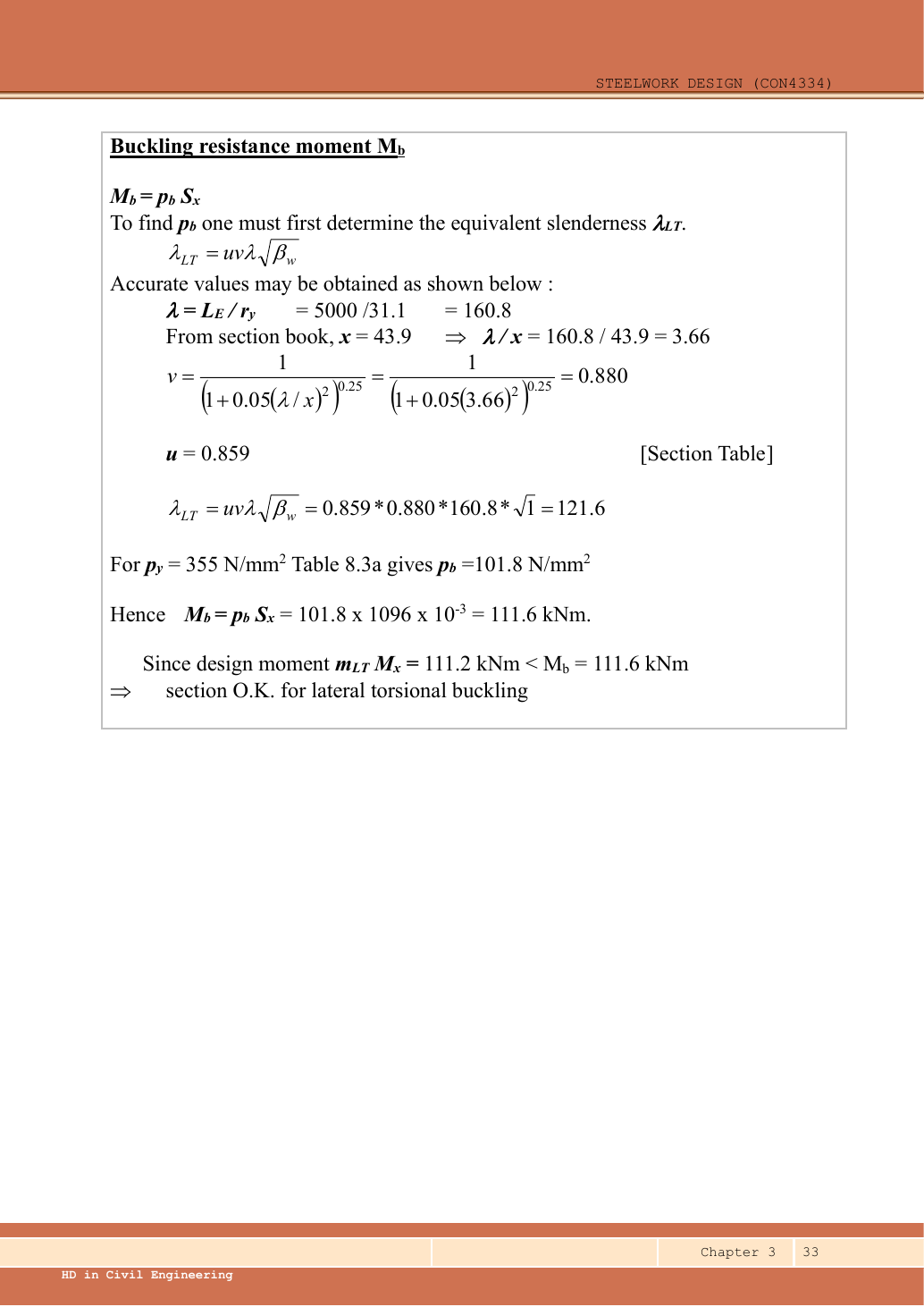
Read the diagram and collect the data
| Input | Source/use |
|---|---|
| Span and load positions | Given dimension chain; central point is at . |
| Lateral model | The question specifies normal loading, end torsional restraint and free in-plane rotation, so . |
| Trial section | The source properties correspond to UB: , , , , , , , , , . |
| Table source | Data File pp.9–10 exact section row; p.5 Table 8.3a strength; p.6 moment factors. |
Before calculating: recognition and strategy
Symmetry makes analysis simple but does not provide lateral restraint. Check the entire length for LTB. Because there are several point loads plus a UDL, the general quarter-point moment factor is appropriate. The result is close to the resistance, so use actual and and interpolate without early rounding.
1. Ultimate loading
Animation labFrom characteristic to design load
Supplement to the original lesson. Enable JavaScript to play, step through calculations and rotate 3D models. The following explanation remains readable offline.
- G is permanent load; Q is imposed load. A surface load and a line load also have different units.
- This illustration uses the course gravity case . Other combinations in the original text retain their own factors.
- For illustrative , change Q and watch each separate contribution.
- Do not carry this ULS total automatically into deflection. Follow the stated SLS load case.
2. Reactions, moment and quarter-point ordinates
Simple explanation: Why reactions balance the loads
Think of a seesaw that must neither fall nor turn.
- Upward and downward forces must balance.
- Take moments about a support to eliminate its reaction.
- Use perpendicular distance from the point to the force line.
Remember: A lateral restraint is not automatically a vertical support.
The lower three-quarter point is at . The equality to follows from the symmetric loading; alternatively include both loads to its left in the free body. No moment contribution is assigned to a load lying to the right of the cut.
Animation labRead the moment shape within one segment
Supplement to the original lesson. Enable JavaScript to play, step through calculations and rotate 3D models. The following explanation remains readable offline.
- Moment ordinates must belong to the same effective unbraced segment.
- Same-side and reverse-curvature diagrams have different signed end ratios.
- The markers show ¼, ½ and ¾ of this segment, not of the entire beam.
- LTB and column flexural factors are different. Preserve their individual bounds and coefficient sets.
3. Trial section and section moment capacity
A small section satisfying M/pᵧ alone would not necessarily pass LTB. The chosen section is a verified trial, not a proof that every lighter section fails.
Animation labCompression and tension across a section
Supplement to the original lesson. Enable JavaScript to play, step through calculations and rotate 3D models. The following explanation remains readable offline.
- For sagging, the top flange is in compression and the bottom in tension; hogging reverses this.
- Elastic bending stress varies with distance from the neutral axis: .
- The section class governs whether elastic, plastic or effective properties may be used.
- Use the shear at the section under examination; the largest shear elsewhere is not automatically coexistent.
4. Section class and shear-web threshold
Animation labWhy thin elements buckle locally
Supplement to the original lesson. Enable JavaScript to play, step through calculations and rotate 3D models. The following explanation remains readable offline.
- The flange outstand and web have different widths, thicknesses and edge support conditions.
- A thinner plate can wrinkle locally before the complete member loses stability.
- Class 1 allows plastic rotation; Class 2 reaches plastic resistance; Class 3 reaches elastic resistance; Class 4 requires effective properties.
- Check every relevant compression element with the supplied limits and stress distribution. The deformation shown is qualitative.
5. Shear and low-shear bending applicability
Animation labSee shear in the web
Supplement to the original lesson. Enable JavaScript to play, step through calculations and rotate 3D models. The following explanation remains readable offline.
- Internal shear keeps the two sides of the cut in vertical equilibrium.
- For the course’s common I-section case, the web provides the principal shear area; use the specified definition.
- A slender web may require a different shear-buckling route before a simple shear-resistance formula is used.
- Use where applicable in the course. Convert N to kN before comparing with design shear.
6. Equivalent moment from Table 8.4b
Simple explanation: Why the shape of the moment diagram matters
The same peak moment is more demanding when a long region stays near that peak.
- Use the diagram of this unrestrained segment.
- Choose the applicable course sketch or quarter-point rule.
- Apply its factor to the demand, following the stated check.
Remember: Column flexural-buckling factors and LTB factors are not interchangeable.
This factor applies to member LTB only. The cross-section still must carry the actual .
Animation labRead the moment shape within one segment
Supplement to the original lesson. Enable JavaScript to play, step through calculations and rotate 3D models. The following explanation remains readable offline.
- Moment ordinates must belong to the same effective unbraced segment.
- Same-side and reverse-curvature diagrams have different signed end ratios.
- The markers show ¼, ½ and ¾ of this segment, not of the entire beam.
- LTB and column flexural factors are different. Preserve their individual bounds and coefficient sets.
7. Effective length and equivalent slenderness
Simple explanation: Which length belongs in the calculation?
A sideways tie can shorten the buckling region without shortening the beam’s vertical span.
- Separate vertical-support spacing from lateral-restraint spacing.
- Apply the course rule for the actual end restraint and loading.
- Keep the original vertical load analysis unless its supports change.
Remember: Restraints in one direction may not restrain the other direction.
The source rounds to and to , obtaining . Both approaches pass, but the exact values avoid losing the small margin in this example.
Animation labA beam bends sideways and twists
Supplement to the original lesson. Enable JavaScript to play, step through calculations and rotate 3D models. The following explanation remains readable offline.
- For the illustrated sagging beam the top flange is compressed.
- The unrestrained compression flange can move sideways while the complete cross-section twists.
- Only effective restraints divide the member into unbraced segments. They do not automatically add vertical supports.
- Use the segment effective length, section properties and matching moment factor. This is an exaggerated mode shape, not a calculated displacement.
8. Interpolate strength and compare
Simple explanation: A beam can escape sideways
The compressed flange can move sideways while the section twists.
- Divide the beam at effective lateral restraints.
- Use each segment’s effective length to obtain its buckling resistance.
- Compare that resistance with the segment’s equivalent moment demand.
Remember: A section bending check alone does not check lateral-torsional buckling.
The lecturer’s rounded route gives pᵦ=101.8 and Mᵦ=111.6 kNm against , also a pass. Do not claim a large reserve. The illustrated solution checks shear, section bending and LTB; bearing dimensions are absent. The characteristic imposed load arrangement is known, but a finish limit is not specified in this example’s question. Those additional design conditions must be supplied before a blanket full-design conclusion.
Animation labA beam bends sideways and twists
Supplement to the original lesson. Enable JavaScript to play, step through calculations and rotate 3D models. The following explanation remains readable offline.
- For the illustrated sagging beam the top flange is compressed.
- The unrestrained compression flange can move sideways while the complete cross-section twists.
- Only effective restraints divide the member into unbraced segments. They do not automatically add vertical supports.
- Use the segment effective length, section properties and matching moment factor. This is an exaggerated mode shape, not a calculated displacement.
Compact exam answer
Use S355 UB, Class 1. Each ,,,. ,. ; , demand . , , ; interpolate . ; LTB passes by only a small margin.
Mistakes to avoid
- Point-load positions do not imply intermediate restraints.
- Use quarter points , not the load positions .
- Read pᵦ using λᴸᵀ, not .
- Do not round a narrow pass into an unsupported generous margin.
Procedure for an unfamiliar variant
- Identify the vertical supports, span, lateral restraints and individual load positions.
- Keep dead and imposed loads separate; form the required ultimate and serviceability cases.
- Find reactions and the maximum shear/moment by equilibrium, with units.
- Choose a section-table row, confirm thickness-dependent strength, and classify both flange and web.
- Check shear and bending; add segment LTB where restraint is discrete.
- Complete the requested web and deflection checks; state the governing result and any missing data.
Independent self-check
Try it yourself. Invented variant: all ultimate loads increase by , with geometry and section unchanged. Does the LTB check still pass?
Reveal answer and reasoning
The moment shape and mᴸᵀ stay unchanged; resistance stays . Demand becomes , exceeding resistance. The beam fails LTB even though section bending and shear have ample reserve.
Animation labRead the moment shape within one segment
Supplement to the original lesson. Enable JavaScript to play, step through calculations and rotate 3D models. The following explanation remains readable offline.
- Moment ordinates must belong to the same effective unbraced segment.
- Same-side and reverse-curvature diagrams have different signed end ratios.
- The markers show ¼, ½ and ¾ of this segment, not of the entire beam.
- LTB and column flexural factors are different. Preserve their individual bounds and coefficient sets.
Animation labFollow the calculation sequence
Supplement to the original lesson. Enable JavaScript to play, step through calculations and rotate 3D models. The following explanation remains readable offline.
- Locate the load, supports, connection geometry and any stated assumptions.
- Keep given values, table lookups and calculated values distinct; reconcile their units.
- The calculation player steps through the existing expressions in their original order.
- Compare demand with resistance or the relevant limit. Keep missing inputs and conditional conclusions explicit.
Practise this chapter: tutorials, assignments and past-paper answers →
Recent-paper practice for this chapter
- 2024 PTE · Compulsory floor beams
- 2024 PTE · LTB beam
- 2023 FT/PTD · 2023 AQ1 — floor beams and fire protection
- 2023 FT/PTD · 2023 FT/PTD BQ4 — overhang and LTB
- 2023 PTE · Compulsory floor beams
- 2023 PTE · LTB beam
- 2022 FT/PTDR · 2022 AQ1 — floor beams and fire protection
- 2022 FT/PTDR · 2022 BQ3 — two point loads and LTB segments