Columns: buckling, eccentric reactions and combined forces
Open “Animation lab” beside a teaching step for a visual explanation or a walkthrough of its original expressions. Models are illustrative; source answers remain unchanged.
Need a simpler picture? Open “Simple explanation” beside a difficult step. These optional notes do not replace the full solution.
A compressed column can fail by local plate buckling, cross-section yielding, or overall member buckling. Passing one does not prove the others. This chapter follows LectureNotes/Ch 4_Column.pdf and the supplied HK2011 tables. The numerical design scope is non-sway columns; sway theory is explained for recognition because it appears in the lectures.
Lecture examples are included immediately after the relevant concepts. Expand an example to read its complete diagram, working, exam answer and self-check here.
1. Effective length belongs to an axis and a restraint model
Simple explanation: Why a long column can fail before crushing
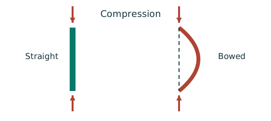
Push a long thin ruler from both ends: it may bow sideways first.
- Find effective length and radius of gyration for each axis.
- Calculate slenderness for both directions.
- Use the appropriate buckling curve before forming resistance.
Remember: Compare the final resistances; slenderness alone may not identify the controlling axis.
Slenderness measures how long and weak a member is in a particular buckling direction: λ=Lᴱ/. Radius of gyration describes how far area lies from that bending axis. Larger gives a smaller slenderness; a weak-axis tie can improve resistance without changing the steel section. It only helps the direction it actually restrains.
| Idealized restraint pattern in Table 8.6 | Theoretical | Recommended when ideal conditions are approximated |
|---|---|---|
| Both ends fixed against rotation and translation | ||
| One end fixed, other pinned; translation prevented | ||
| One end fixed, other rotation-fixed but translation-free | ||
| Both ends pinned, translation prevented | ||
| Fixed-free cantilever | ||
| Source sixth pattern with partial rotational restraint and free translation at top | Not specified |
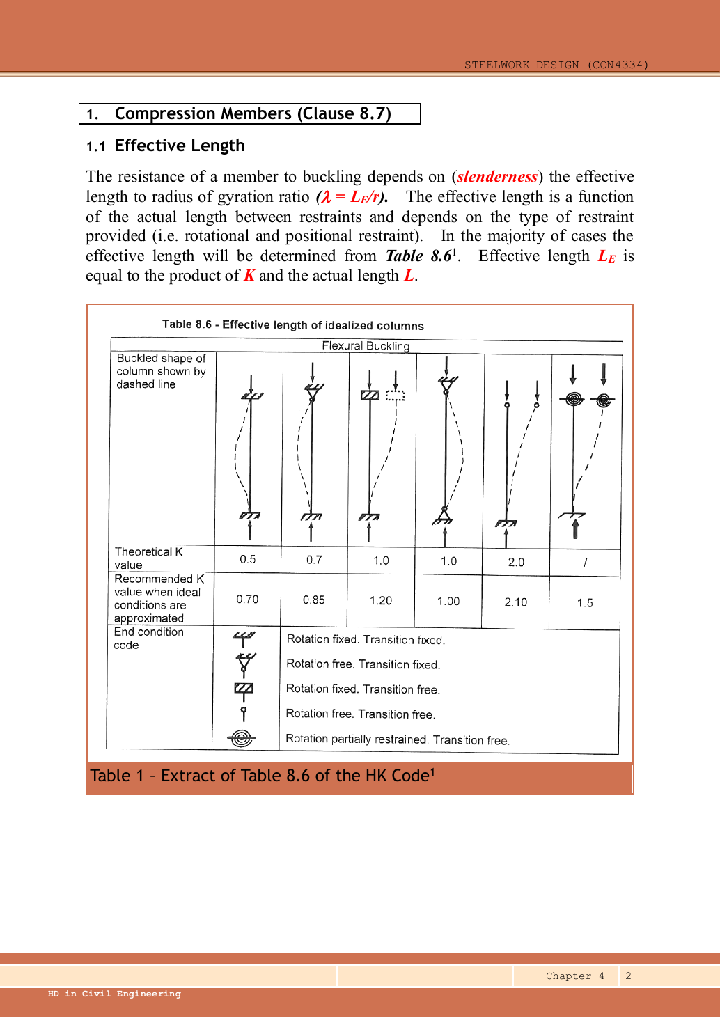
Use the question’s explicitly given effective length if present. Otherwise choose the source’s recommended factor for the modeled conditions, as the examples do. Do not use textbook theoretical where the worked course method uses . Pin symbols indicate free rotation, not free lateral translation. Keep and in the same units.
Try it yourself. A6 m pinned column has a midheight tie effective only against weak-axis buckling. Find Lᴱx and Lᴱy.
Reveal answer and reasoning
; . Major-axis buckling can still extend over the full height.
Animation labEffective length and buckling axes
Supplement to the original lesson. Enable JavaScript to play, step through calculations and rotate 3D models. The following explanation remains readable offline.
- A column can bow sideways before its section reaches the crushing resistance.
- Each axis has its own radius of gyration and restraint spacing.
- , with compatible length units. A tie affects only the directions it actually restrains.
- Select each buckling curve and compressive strength before forming Pc. The governing axis is determined by resistance, not slenderness alone.
Animation labEffective length and buckling axes
Supplement to the original lesson. Enable JavaScript to play, step through calculations and rotate 3D models. The following explanation remains readable offline.
- A column can bow sideways before its section reaches the crushing resistance.
- Each axis has its own radius of gyration and restraint spacing.
- , with compatible length units. A tie affects only the directions it actually restrains.
- Select each buckling curve and compressive strength before forming Pc. The governing axis is determined by resistance, not slenderness alone.
2. Select the buckling curve before reading compressive strength
Simple explanation: A table lookup needs several keys
A table is like an address: knowing only the street is not enough.
- Select the curve using section type, thickness and axis.
- Select the material-strength column.
- Bracket the slenderness and interpolate if required.
Remember: Do not jump between steel grades or extrapolate past supplied data.
First establish that the section is not slender. For uniform compression the lecture checks flange and web , the semi-compact limits. That permits the gross-area resistance ; it does not assert Class 1. For combined bending and axial force, use the appropriate class limits before claiming plastic bending resistance.
| Section; maximum thickness | Curve about | Curve about |
|---|---|---|
| Rolled I; | ||
| Rolled I; | ||
| Rolled H (UC); | ||
| Rolled H; | ||
| Welded I or H; | ||
| Welded I or H; |
These rows are Table 8.7 in the Data File p.7. The full source on Ch 4 p.4 also covers hollow sections, bars, angles, channels, cover plates and welded boxes. The full table’s notes matter: thickness – permits the specified averaging treatment; fabrication and cover-plate geometry can alter the curve. Do not select a curve solely from steel grade.
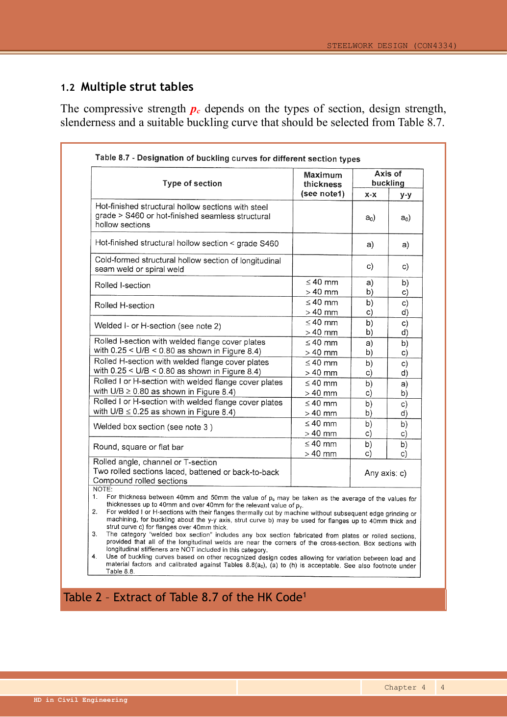
Hot-finished structural hollow sections in steel above S460, or hot-finished seamless hollow sections: /. Hot-finished hollow sections in steel below S460: /. These two source rows say “above” and “below”; neither explicitly assigns exactly S460, so do not invent an equality boundary. Cold-formed hollow sections with longitudinal or spiral welds: /.
Hot-rolled I-sections: thickness uses /; uses /. Hot-rolled H-sections: for the same two thickness intervals, use respectively / and /. Welded I/H-sections: use respectively / and /; also see note 2.
Hot-rolled sections with welded flange cover plates: select the row using the Figure 8.4 ratio . When : for I-sections in the two thickness intervals above, use respectively / and /; for H-sections, use respectively / and /. When : for I/H-sections, use respectively / and /. When : for I/H-sections, use respectively / and /.
Welded box sections: for the two thickness intervals above, use respectively / and /; also see note 3. Round, square or flat bars: use respectively / and /. Hot-rolled angles, channels and tees; two hot-rolled sections connected by lacing, battens or back to back; and built-up hot-rolled sections: for either axis, use .
Note 1: for thickness to , for the same relevant , average the values for thickness not exceeding and thickness exceeding of . Note 2: for welded I/H-section flanges machine flame-cut without subsequent edge grinding or machining, when buckling about the axis, flange thickness not exceeding may use curve ; above that thickness, use . Note 3: “welded box sections” includes boxes assembled from plates or hot-rolled sections with all longitudinal welds near the corners, but excludes boxes with longitudinal stiffeners. Note 4: the source permits curves from other recognised codes when differences in load/material partial factors are addressed and the curves are calibrated against Tables 8.8(a₀), (a) to (h); the Table 8.8 footnote also applies. This does not supply numerical values that can simply be mixed with the course tables.Open full-size image
- Identify section family and fabrication, maximum thickness and buckling axis; choose its curve.
- Confirm pᵧ from grade and thickness. Select that strength column within the appropriate Table 8.8 curve.
- Calculate for that axis and locate bracketing rows. Interpolate ; do not extrapolate beyond supplied tables.
- Compute and ; use the smaller for the flexural compression check.
Check both axes even if rᵧ is smaller: different effective lengths and different curves may change which controls. Data File p.8 supplies S355 curves only over its printed rows; the lecture and 2023 extra data contain further tables. Choose a supplied applicable table and cite it; do not invent a value from the trend.
Column example 1: a pinned column in axial compression
Open this example on its own page
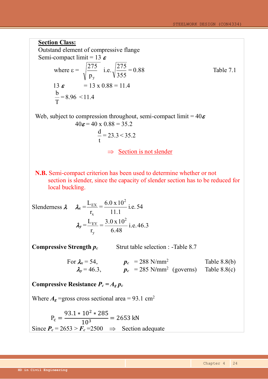
Select a Grade S355 UC for a column pinned at both ends, carrying a design axial compression of . Check the selected section’s compression resistance.
Original source: LectureNotes/Ch 4_Column.pdf — p. 21, p. 22. Values tagged given are in the question or diagram; lookup values come from a named table; calculated values follow from the working; assumptions are stated explicitly.
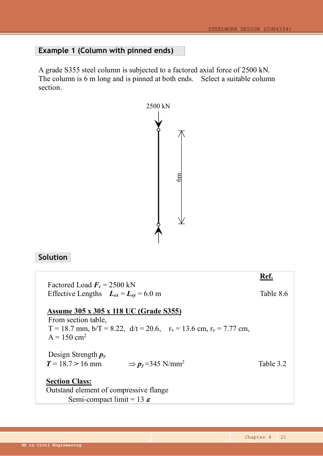
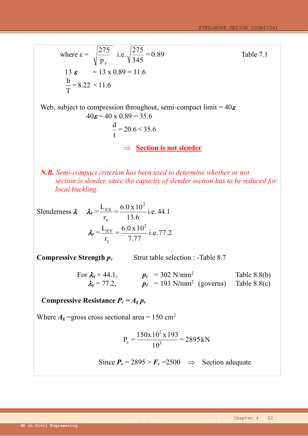
Read the diagram and collect the data
| Input | Source and meaning |
|---|---|
| Design load | Given , already factored; no dead/imposed breakdown is needed. |
| Restraints | Pinned-pinned, translation prevented at ends; Table 8.6 gives in both axes. |
| Selected row | Data File p.11, UC: flange , , , , , . |
| Strength and curves | S355,, giving . Hot-rolled H-section, , so axis uses curve b; axis uses curve c. |
Before calculating: recognition and strategy
There is no stated bending moment, so the core numerical task is axial member buckling. First ensure the local plates are not slender, allowing gross area. Then calculate both axis slendernesses and select the correct curve for each. The area alone is not enough: a long weak column can buckle well before reaching A𝗀pᵧ.
1. Choose a section and confirm its strength
The lecturer selects a trial UC. Its nominal mass is part of the section designation. The strength calculation uses the tabulated gross area . The flange thickness is , falling within the S355 thickness band .
exceeds the load but is not the member resistance. Proceed to local-slenderness and overall-buckling checks.
Animation labEffective length and buckling axes
Supplement to the original lesson. Enable JavaScript to play, step through calculations and rotate 3D models. The following explanation remains readable offline.
- A column can bow sideways before its section reaches the crushing resistance.
- Each axis has its own radius of gyration and restraint spacing.
- , with compatible length units. A tie affects only the directions it actually restrains.
- Select each buckling curve and compressive strength before forming Pc. The governing axis is determined by resistance, not slenderness alone.
2. Establish a non-slender section
Simple explanation: A thin part can wrinkle first
A thin plate may wrinkle before the whole steel member reaches its intended resistance.
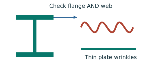
- Check flange and web slenderness using their own definitions.
- Compare each ratio with the correct class limits.
- The less favourable element determines the section class.
Remember: Bending limits and uniform-compression limits are different.
This establishes Class 3 or better, not necessarily a plastic flange. The pure-compression example does not need plastic bending resistance; checking the non-slender boundary is sufficient for its stated method.
Animation labWhy thin elements buckle locally
Supplement to the original lesson. Enable JavaScript to play, step through calculations and rotate 3D models. The following explanation remains readable offline.
- The flange outstand and web have different widths, thicknesses and edge support conditions.
- A thinner plate can wrinkle locally before the complete member loses stability.
- Class 1 allows plastic rotation; Class 2 reaches plastic resistance; Class 3 reaches elastic resistance; Class 4 requires effective properties.
- Check every relevant compression element with the supplied limits and stress distribution. The deformation shown is qualitative.
3. Calculate slenderness about both axes
Simple explanation: Why a long column can fail before crushing
Push a long thin ruler from both ends: it may bow sideways first.
- Find effective length and radius of gyration for each axis.
- Calculate slenderness for both directions.
- Use the appropriate buckling curve before forming resistance.
Remember: Compare the final resistances; slenderness alone may not identify the controlling axis.
The smaller weak-axis radius makes its slenderness much larger. Still read both curves rather than assuming the larger slenderness by itself proves which resistance controls.
Animation labEffective length and buckling axes
Supplement to the original lesson. Enable JavaScript to play, step through calculations and rotate 3D models. The following explanation remains readable offline.
- A column can bow sideways before its section reaches the crushing resistance.
- Each axis has its own radius of gyration and restraint spacing.
- , with compatible length units. A tie affects only the directions it actually restrains.
- Select each buckling curve and compressive strength before forming Pc. The governing axis is determined by resistance, not slenderness alone.
4. Read and interpolate the two compressive strengths
Simple explanation: A table lookup needs several keys
A table is like an address: knowing only the street is not enough.
- Select the curve using section type, thickness and axis.
- Select the material-strength column.
- Bracket the slenderness and interpolate if required.
Remember: Do not jump between steel grades or extrapolate past supplied data.
Table 8.7, rolled H section with maximum thickness : uses 8.8(b), uses 8.8(c). In each use the pᵧ=345 column of Data File p.8.
The source rounds these to and . The minor axis has the smaller and controls for the same area.
Animation labEffective length and buckling axes
Supplement to the original lesson. Enable JavaScript to play, step through calculations and rotate 3D models. The following explanation remains readable offline.
- A column can bow sideways before its section reaches the crushing resistance.
- Each axis has its own radius of gyration and restraint spacing.
- , with compatible length units. A tie affects only the directions it actually restrains.
- Select each buckling curve and compressive strength before forming Pc. The governing axis is determined by resistance, not slenderness alone.
5. Form resistances and conclude
Using the lecturer’s rounded gives , agreeing with the original answer. The governing failure mode is minor-axis overall buckling, not yielding of the full gross area.
Animation labEffective length and buckling axes
Supplement to the original lesson. Enable JavaScript to play, step through calculations and rotate 3D models. The following explanation remains readable offline.
- A column can bow sideways before its section reaches the crushing resistance.
- Each axis has its own radius of gyration and restraint spacing.
- , with compatible length units. A tie affects only the directions it actually restrains.
- Select each buckling curve and compressive strength before forming Pc. The governing axis is determined by resistance, not slenderness alone.
Compact exam answer
Select S355 UC; , giving . ,, non-slender.,,. Curves b/c give respectively , . , adequate. Rounded source result .
Mistakes to avoid
- Do not use solely because the steel is S355.
- Do not halve the effective length just because both ends are supported.
- Do not use the same strut curve for both UC axes.
- Do not treat the lower reaction arrow as a second applied load.
Procedure for an unfamiliar variant
- Identify axial load, any moments, actual length and restraints in each axis.
- Choose/read a section and confirm strength from the actual thickness.
- Check the appropriate flange and web local-slenderness limits.
- Find and separately; select each axis curve and interpolate .
- Calculate both axial resistances and identify the governing axis.
- If moments exist, complete section, flexural and axial/LTB interactions using their own capacities and moment definitions.
Independent self-check
Try it yourself. Invented variant: the same column now carries design axial compression, with the same length and restraints. Does it pass?
Reveal answer and reasoning
No. Non-slender classification and buckling resistance are unchanged. Utilisation. The gross squash resistance cannot override the member buckling failure.
Animation labEffective length and buckling axes
Supplement to the original lesson. Enable JavaScript to play, step through calculations and rotate 3D models. The following explanation remains readable offline.
- A column can bow sideways before its section reaches the crushing resistance.
- Each axis has its own radius of gyration and restraint spacing.
- , with compatible length units. A tie affects only the directions it actually restrains.
- Select each buckling curve and compressive strength before forming Pc. The governing axis is determined by resistance, not slenderness alone.
Column example 2: a weak-axis tie permits a lighter section
Open this example on its own page
Repeat the axial-column design with a pinned column and an effective midheight tie against weak-axis buckling. Select and check a Grade S355 UC.
Original source: LectureNotes/Ch 4_Column.pdf — p. 23, p. 24. Values tagged given are in the question or diagram; lookup values come from a named table; calculated values follow from the working; assumptions are stated explicitly.
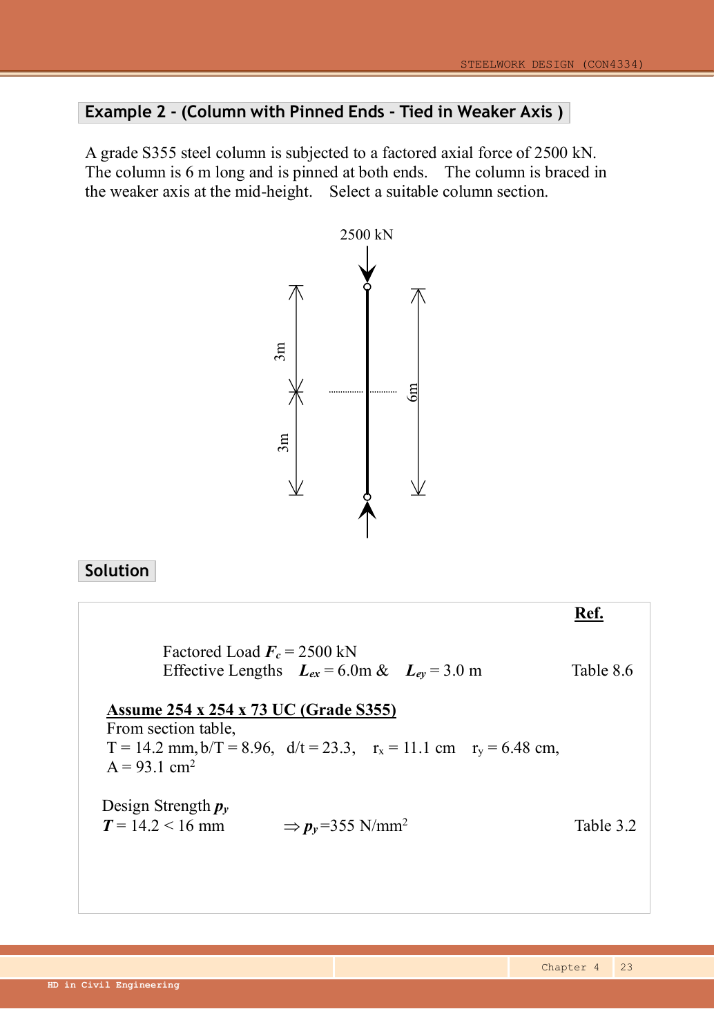
Read the diagram and collect the data
| Input | Origin |
|---|---|
| Axial force | Given design compression. |
| Direction of tie | Question states weak direction: shorten -axis buckling length only. |
| Trial section | Data File p.11, UC: , , , , , . |
| Tables | pᵧ355 because ; rolled H uses curves b/c. |
Before calculating: recognition and strategy
Compare this to Example 1: restraints can be as important as area. The weak-axis tie reduces its unbraced length from to . A smaller column is now possible, but after changing section both radii, the area and the thickness-dependent strength must be reread. Do not reuse Example 1’s section properties.
1. Set each effective length
Simple explanation: Why a long column can fail before crushing
Push a long thin ruler from both ends: it may bow sideways first.
- Find effective length and radius of gyration for each axis.
- Calculate slenderness for both directions.
- Use the appropriate buckling curve before forming resistance.
Remember: Compare the final resistances; slenderness alone may not identify the controlling axis.
A horizontal positional restraint suppresses a buckling displacement. It does not support half the vertical load or create a new compression case.
Animation labEffective length and buckling axes
Supplement to the original lesson. Enable JavaScript to play, step through calculations and rotate 3D models. The following explanation remains readable offline.
- A column can bow sideways before its section reaches the crushing resistance.
- Each axis has its own radius of gyration and restraint spacing.
- , with compatible length units. A tie affects only the directions it actually restrains.
- Select each buckling curve and compressive strength before forming Pc. The governing axis is determined by resistance, not slenderness alone.
2. Trial UC
These values come from the same exact section row on Data File p.11. This lighter trial is the one selected in the lecture.
Animation labEffective length and buckling axes
Supplement to the original lesson. Enable JavaScript to play, step through calculations and rotate 3D models. The following explanation remains readable offline.
- A column can bow sideways before its section reaches the crushing resistance.
- Each axis has its own radius of gyration and restraint spacing.
- , with compatible length units. A tie affects only the directions it actually restrains.
- Select each buckling curve and compressive strength before forming Pc. The governing axis is determined by resistance, not slenderness alone.
3. Check local slenderness
Animation labWhy thin elements buckle locally
Supplement to the original lesson. Enable JavaScript to play, step through calculations and rotate 3D models. The following explanation remains readable offline.
- The flange outstand and web have different widths, thicknesses and edge support conditions.
- A thinner plate can wrinkle locally before the complete member loses stability.
- Class 1 allows plastic rotation; Class 2 reaches plastic resistance; Class 3 reaches elastic resistance; Class 4 requires effective properties.
- Check every relevant compression element with the supplied limits and stress distribution. The deformation shown is qualitative.
4. Slenderness for the tied and untied directions
Now exceeds . That alone does not prove the axis controls because its curve b is more favourable than the weak-axis curve c.
Animation labEffective length and buckling axes
Supplement to the original lesson. Enable JavaScript to play, step through calculations and rotate 3D models. The following explanation remains readable offline.
- A column can bow sideways before its section reaches the crushing resistance.
- Each axis has its own radius of gyration and restraint spacing.
- , with compatible length units. A tie affects only the directions it actually restrains.
- Select each buckling curve and compressive strength before forming Pc. The governing axis is determined by resistance, not slenderness alone.
5. Interpolate each curve
Simple explanation: A value between two table rows
Move the same fraction of the way across both number ranges.
- Choose the correct table, curve and strength column first.
- Find how far your input lies between the two rows.
- Apply that fraction to the change between their answers.
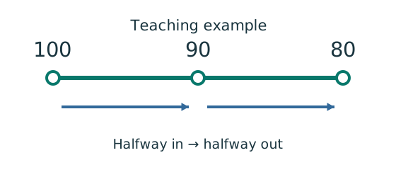
Remember: Teaching example: halfway between outputs 100 and 80 gives 90.
Use Table 8.8(b), pᵧ355 for and Table 8.8(c), pᵧ355 for .
Despite its smaller slenderness, the weak axis gives the slightly smaller strength. The source values and are rounded representations.
Animation labEffective length and buckling axes
Supplement to the original lesson. Enable JavaScript to play, step through calculations and rotate 3D models. The following explanation remains readable offline.
- A column can bow sideways before its section reaches the crushing resistance.
- Each axis has its own radius of gyration and restraint spacing.
- , with compatible length units. A tie affects only the directions it actually restrains.
- Select each buckling curve and compressive strength before forming Pc. The governing axis is determined by resistance, not slenderness alone.
6. Check the controlling resistance
The original rounds to , giving , printed . The exact interpolation gives . The tie makes the trial adequate where the untied example used . This conclusion assumes the tie provides the stated effective restraint; tie design itself is not part of this question.
Animation labEffective length and buckling axes
Supplement to the original lesson. Enable JavaScript to play, step through calculations and rotate 3D models. The following explanation remains readable offline.
- A column can bow sideways before its section reaches the crushing resistance.
- Each axis has its own radius of gyration and restraint spacing.
- , with compatible length units. A tie affects only the directions it actually restrains.
- Select each buckling curve and compressive strength before forming Pc. The governing axis is determined by resistance, not slenderness alone.
Compact exam answer
Use S355 UC,; under the , limits, it is non-slender., ; , . Curves b/c give , . , adequate. Rounded source resistance .
Mistakes to avoid
- The tie changes only its effective buckling direction.
- Use the full axial force in both portions.
- Compare actual values, not slenderness alone.
- Reclassify after selecting a lighter section.
Procedure for an unfamiliar variant
- Identify axial load, any moments, actual length and restraints in each axis.
- Choose/read a section and confirm strength from the actual thickness.
- Check the appropriate flange and web local-slenderness limits.
- Find and separately; select each axis curve and interpolate .
- Calculate both axial resistances and identify the governing axis.
- If moments exist, complete section, flexural and axial/LTB interactions using their own capacities and moment definitions.
Independent self-check
Try it yourself. Invented variant: remove the weak-axis tie but retain UC. Find the weak-axis slenderness and estimate its supplied-table resistance.
Reveal answer and reasoning
. Curve c,pᵧ355: row gives and gives , so . , much less than . The untied version fails.
Animation labEffective length and buckling axes
Supplement to the original lesson. Enable JavaScript to play, step through calculations and rotate 3D models. The following explanation remains readable offline.
- A column can bow sideways before its section reaches the crushing resistance.
- Each axis has its own radius of gyration and restraint spacing.
- , with compatible length units. A tie affects only the directions it actually restrains.
- Select each buckling curve and compressive strength before forming Pc. The governing axis is determined by resistance, not slenderness alone.
Animation labEffective length and buckling axes
Supplement to the original lesson. Enable JavaScript to play, step through calculations and rotate 3D models. The following explanation remains readable offline.
- A column can bow sideways before its section reaches the crushing resistance.
- Each axis has its own radius of gyration and restraint spacing.
- , with compatible length units. A tie affects only the directions it actually restrains.
- Select each buckling curve and compressive strength before forming Pc. The governing axis is determined by resistance, not slenderness alone.
3. Cross-section capacity: axial force consumes some of the same resistance
Simple explanation: The column needs more than one pass
A slice can be strong while the whole member still buckles.
- Check cross-section compression plus bending.
- Then check the separate member-buckling expressions.
- Keep each moment, factor and resistance in its specified expression.
Remember: The three checks do not share interchangeable denominators.
is design compression at the critical section; and Mᵧ are design moments there, including the specified amplification. is gross area. Each ratio is dimensionless, so keep force units consistent and moment units consistent. Use magnitudes for the conservative linear interaction; moments about perpendicular axes do not cancel. If using maxima from different locations, label the check as a conservative envelope. This lecture expression excludes Class 4 without an appropriate local-buckling treatment.
The minor-axis 1.2pᵧZᵧ ceiling frequently controls UC sections: calculating pᵧSᵧ alone overstates the allowed moment. The axial denominator here is A𝗀pᵧ, not the reduced member resistance .
Animation labA strong slice can belong to an unstable member
Supplement to the original lesson. Enable JavaScript to play, step through calculations and rotate 3D models. The following explanation remains readable offline.
- Combine axial compression and the two bending demands using the specified section resistances.
- The whole member adds effective-length and buckling-curve effects.
- This uses its own moment factor and bending resistance; it is not a copy of the section check.
- Elastic, plastic and buckling resistances are not interchangeable. Read the three original expressions and their first-order/amplified moments.
4. Member buckling: keep the source’s barred quantities distinct
Simple explanation: The column needs more than one pass
A slice can be strong while the whole member still buckles.
- Check cross-section compression plus bending.
- Then check the separate member-buckling expressions.
- Keep each moment, factor and resistance in its specified expression.
Remember: The three checks do not share interchangeable denominators.
The source uses bars to distinguish first-order moments and some resistance definitions. Small overbars can disappear in extracted text, so read the original image. Here “Mᵧ,first” explicitly means the source’s barred Mᵧ. “” and “Mᵧ,amp” include the required amplification. Elastic moment denominators in these member equations are pᵧZ, even for a Class 1 section.
Non-sway flexural-buckling interaction (course Eq.8.80): Combined axial force/LTB (Eq.8.81):
For the non-sway worked method, is the smaller axis resistance based on the stated/computed effective lengths; specifically uses weak-axis buckling. Mᴸᵀ is the amplified major-axis moment governing lateral-torsional resistance, often given separately by an exam question. Do not amplify a supplied “already amplified” Mᴸᵀ twice. The last term of Eq.8.81 uses first-order minor-axis moment in the supplied source; the flexural equation uses the amplified one. This explains the apparently different and values in Example 5.
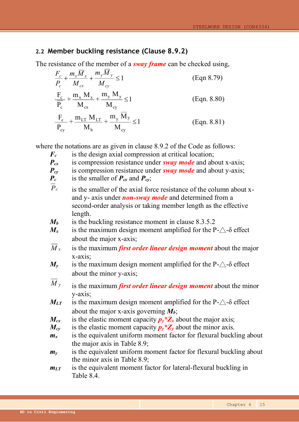
Eqn 8.79: Eqn 8.80: Eqn 8.81: Source definitions: is the design compressive force at the critical location; , are the compression resistances about the two axes in sway mode; is the smaller of these; is the smaller of the two non-sway compression resistances, obtained by second-order analysis or by taking effective length equal to actual member length. is the buckling moment resistance under clause 8.3.5.2. , are the maximum major- and minor-axis design moments already amplified for effects; , are the corresponding first-order linear-analysis moments. is the amplified major-axis moment governing . In this source figure, , denotes elastic moment resistance. , comes from Table 8.9; comes from Table 8.4.Open full-size image
For sway recognition only, Eq.8.79 uses sway-mode compression resistance with first-order end moments, while Eq.8.80 uses the alternative non-sway-mode compression resistance with amplified moments. Eq.8.81 adds axial/LTB interaction. The source explains that different lateral-load/initial-curvature effects can control. Its p.17 explicitly excludes numerical sway-column design from the course; the worked pages therefore use the non-sway branches rather than constructing an unsupported sway analysis.
Animation labA strong slice can belong to an unstable member
Supplement to the original lesson. Enable JavaScript to play, step through calculations and rotate 3D models. The following explanation remains readable offline.
- Combine axial compression and the two bending demands using the specified section resistances.
- The whole member adds effective-length and buckling-curve effects.
- This uses its own moment factor and bending resistance; it is not a copy of the section check.
- Elastic, plastic and buckling resistances are not interchangeable. Read the three original expressions and their first-order/amplified moments.
5. Non-sway, sway and ultra-sensitive frames
| Source analysis route | Non-sway | Sway | Ultra-sensitive |
|---|---|---|---|
| Ordinary course route | |||
| Advanced-analysis classification quoted by lecture |
is the elastic critical load factor: the multiple of the applied loading at which an elastic instability mode occurs. It is not the member slenderness λ=Lᴱ/r. Non-sway classification permits the stated global simplification; local member amplification may still be needed. For ultra-sensitive frames the lecture requires second-order or advanced analysis. Bracing is the physical system restraining sway; the classification checks how sensitive the modeled structure is.
Animation labRestraints, sway and imperfections
Supplement to the original lesson. Enable JavaScript to play, step through calculations and rotate 3D models. The following explanation remains readable offline.
- A frame needs a defined path for horizontal force as well as gravity.
- Pinned joints alone do not provide frame moment resistance; sway restraint needs a real structural system.
- Diagonal bracing carries horizontal action through axial forces. This sketch does not assign a numerical frame classification.
- Use the specified imperfection/notional-force model and critical-load criteria. Avoid counting alternative imperfection models twice.
6. Why moments increase under compression
Simple explanation: Moving sideways gives the load a new lever arm
Once a compressed member moves sideways, the same compression creates extra moment.
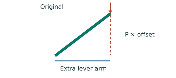
- P–Δ concerns overall frame or storey movement.
- P–δ concerns bowing relative to the member’s end line.
- Amplify only the first-order moments specified by the method.
Remember: Do not amplify a moment that the question already gives as amplified.
A compression force acting through a lateral displacement creates additional moment. Capital usually denotes frame/storey sway; small denotes member curvature. Second-order analysis can include these effects directly. If the exercise instead gives amplification factors, multiply the appropriate first-order moment once.
Global amplification factor: Member amplification factor:
is the factored vertical load at and above the storey; Fᴺ is the notional horizontal load; is storey height; δᴺ is relative storey displacement caused by Fᴺ. The lecture uses the larger relevant global/member factor for its general discussion. For non-sway member design it specifies the local member factor. Use a consistent force/length system so both denominator ratios are dimensionless. A nonpositive denominator does not mean a negative useful amplification: the approximation has reached/breached its instability condition.
Try it yourself. Invented arithmetic: , Fᴺ/Fᵥ=0.005, δᴺ=2 mm. Find and the global factor.
Reveal answer and reasoning
. The ordinary route is at the non-sway boundary. The displayed global factor is ; a separate member effect may still govern.
Animation labSeparate P–Δ from P–δ
Supplement to the original lesson. Enable JavaScript to play, step through calculations and rotate 3D models. The following explanation remains readable offline.
- The dashed line marks the original frame position; axial compression acts downwards.
- Global displacement Δ creates the additional moment PΔ.
- Local displacement δ is measured from the line joining the displaced ends, and adds Pδ.
- Follow the original analysis route. Do not amplify an already amplified moment or confuse critical-load factor with member slenderness.
Animation labSeparate P–Δ from P–δ
Supplement to the original lesson. Enable JavaScript to play, step through calculations and rotate 3D models. The following explanation remains readable offline.
- The dashed line marks the original frame position; axial compression acts downwards.
- Global displacement Δ creates the additional moment PΔ.
- Local displacement δ is measured from the line joining the displaced ends, and adds Pδ.
- Follow the original analysis route. Do not amplify an already amplified moment or confuse critical-load factor with member slenderness.
7. Flexural moment factors are not the LTB factors
Simple explanation: Similar-looking moment factors come from different tables
Two recipes can use the same ingredients but different amounts.
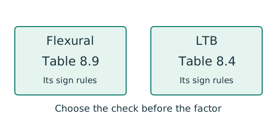
- Identify flexural buckling or lateral-torsional buckling first.
- Read the actual moment diagram, including any change of sign.
- Use that check’s table and its own sign and minimum-factor rules.
Remember: Table 8.9 flexural factors are not Table 8.4 LTB factors.
For an end-moment-only segment, read Table 8.9 with the signed internal end-moment ratio . positive means the BMD stays on the same side; negative means it reverses. The lecture’s column-end applied-arrow convention gives ; confirm the actual arrow/BMD rather than applying that minus sign blindly to internal BMD ordinates.
When : .
When : .
For example, ; .
But Table 8.4a for LTB, at , gives .
The two tables differ especially for reversing bending. They also have different general quarter-point formulas. For Table 8.9:
and are quarter-point moments; is mid-length moment. is the maximum moment magnitude in the central half. If the three ordinates lie on one side, take them positive; if they straddle the axis, choose the positive side that gives the larger . and are always positive. This sign rule differs from Table 8.4b, which uses all magnitudes. The lecture’s special flexural cases give for one central point, for a UDL, for three equal equally spaced points and for the pictured two equal points; match the drawing before using them.
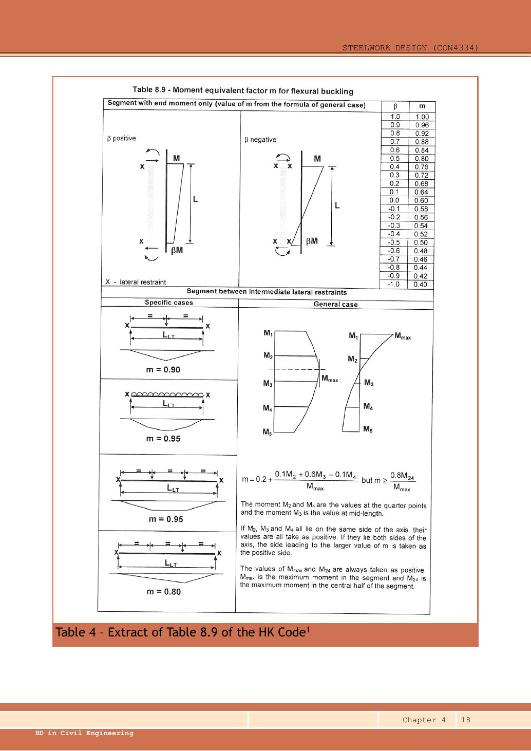
,,,,,,,,,,,,,,,,,,,,.
The special cases at lower left, from top to bottom, are: one point load at midspan, ; UDL, ; three equal, equally spaced point loads, ; two equal point loads at the third points, . In the lower-right sketch, , are the ends; , are the quarter points; is the midpoint. The source expression is:but . If all three sampled moments lie on the same side, take them positive. If they lie on different sides, choose as positive the side producing the larger . , are both positive: respectively the maximum moment over the whole segment and over its central half.Open full-size image
Column example 5: axial load plus biaxial end moments
Open this example on its own page
Check a UC S355 column in a braced non-sway frame, long, fixed at one end and pinned at the other. Design compression is . First-order factored end moments are (top/bottom)=/ and Mᵧ(top/bottom)=/. Amplification factors are about and about . The given amplified Mᴸᵀ=86.4 kNm has the same distribution as .
Original source: LectureNotes/Ch 4_Column.pdf — p. 36, p. 37, p. 38. Values tagged given are in the question or diagram; lookup values come from a named table; calculated values follow from the working; assumptions are stated explicitly.
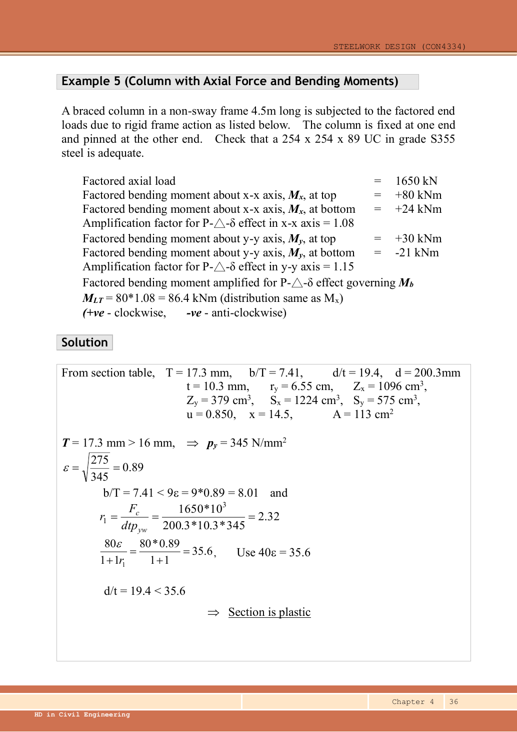
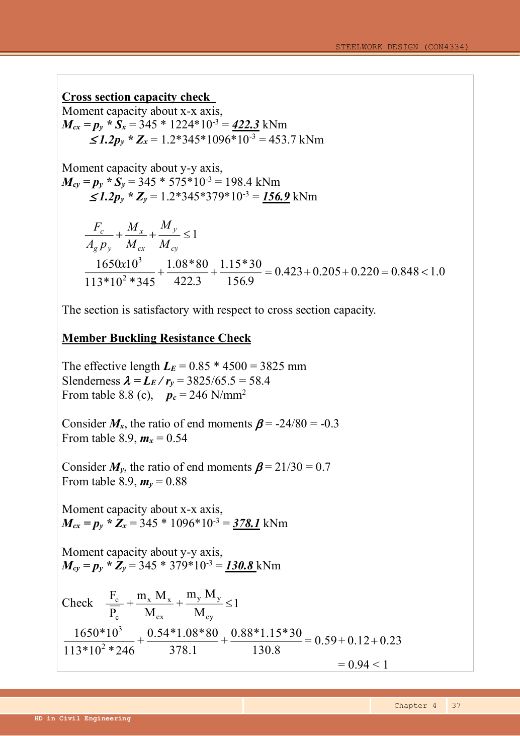
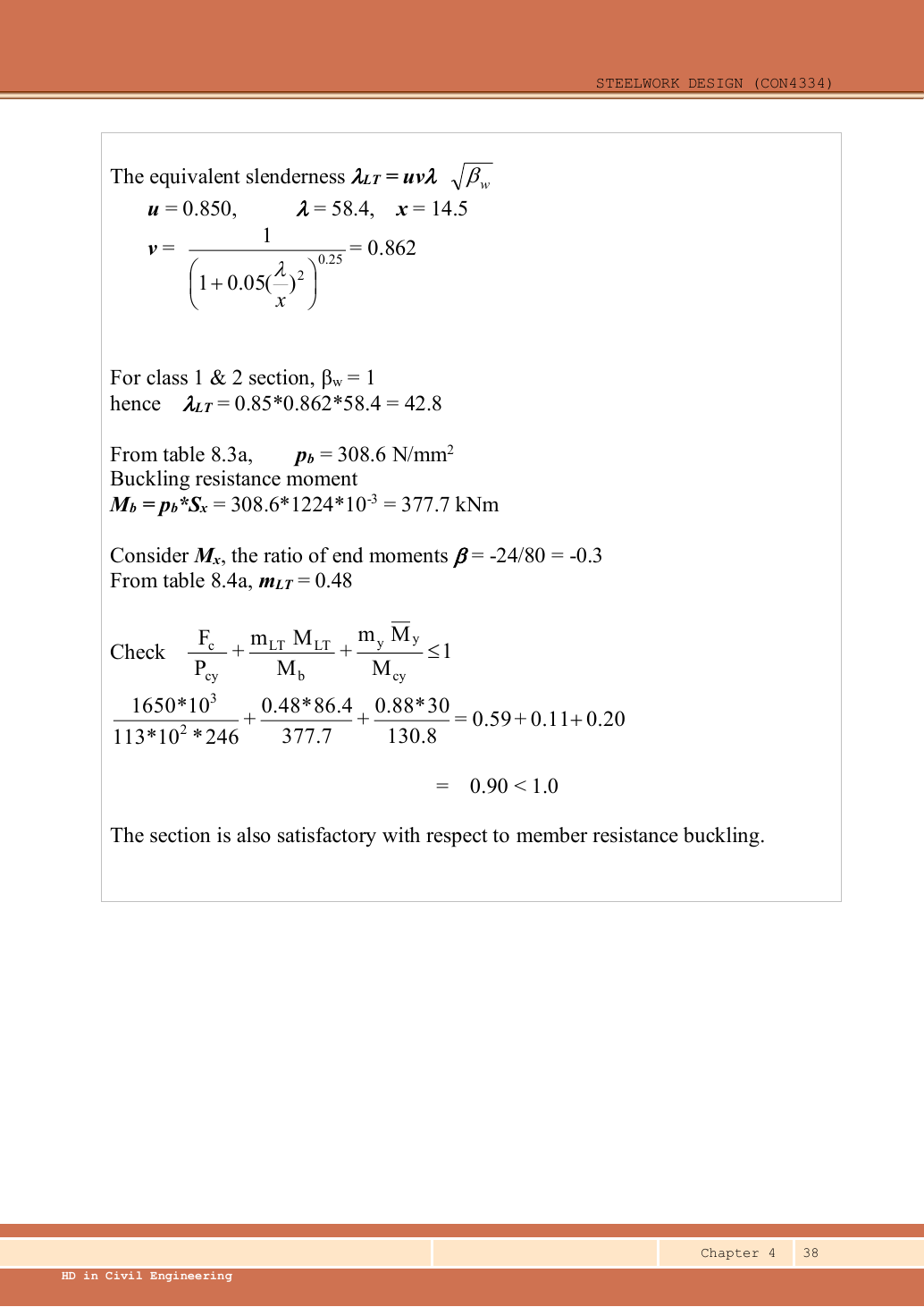
Read the diagram and collect the data
| Input | Meaning/value source |
|---|---|
| End moments | Given applied-arrow convention: / about ; / about . Convert to the Table 8.9 internal-diagram ratio. |
| Amplification | Given and ; Mᴸᵀ86.4 already includes amplification. |
| Section row | Data File p.11, UC: , , ; , ; , ; ; , , , ; , . |
| Restraint/curve choices | Table 8.6 recommended fixed/pinned K0.85; rolled H uses b about ,c about . |
Before calculating: recognition and strategy
This is continuous-frame end-moment design, so use the full LTB procedure and moment factors from the separate flexural/LTB tables. Check three things: local section interaction, flexural member interaction, and axial/LTB interaction. The section moment denominator is capped plastic resistance, whereas the member denominators are elastic pᵧZ. The source’s LTB minor-axis term uses first-order Mᵧ; its flexural term uses amplified Mᵧ.
1. Strength, combined-stress classification and moments
The raw exceeds because the axial load is divided by the web’s area, not total section area. The course classification parameter is bounded; this does not mean gross-area compression exceeds capacity.
Animation labWhy thin elements buckle locally
Supplement to the original lesson. Enable JavaScript to play, step through calculations and rotate 3D models. The following explanation remains readable offline.
- The flange outstand and web have different widths, thicknesses and edge support conditions.
- A thinner plate can wrinkle locally before the complete member loses stability.
- Class 1 allows plastic rotation; Class 2 reaches plastic resistance; Class 3 reaches elastic resistance; Class 4 requires effective properties.
- Check every relevant compression element with the supplied limits and stress distribution. The deformation shown is qualitative.
2. Cross-section interaction
Simple explanation: The column needs more than one pass
A slice can be strong while the whole member still buckles.
- Check cross-section compression plus bending.
- Then check the separate member-buckling expressions.
- Keep each moment, factor and resistance in its specified expression.
Remember: The three checks do not share interchangeable denominators.
Both maximum moment magnitudes occur at the top in the given load schedule, so they coexist with the stated compression there. The minor-axis ceiling is the governing branch for .
Animation labA strong slice can belong to an unstable member
Supplement to the original lesson. Enable JavaScript to play, step through calculations and rotate 3D models. The following explanation remains readable offline.
- Combine axial compression and the two bending demands using the specified section resistances.
- The whole member adds effective-length and buckling-curve effects.
- This uses its own moment factor and bending resistance; it is not a copy of the section check.
- Elastic, plastic and buckling resistances are not interchangeable. Read the three original expressions and their first-order/amplified moments.
3. Effective length and both axial buckling resistances
Select curve b for and c for ; both use pᵧ345. The source shows only the controlling result; the lookup below completes the omitted comparison.
Animation labEffective length and buckling axes
Supplement to the original lesson. Enable JavaScript to play, step through calculations and rotate 3D models. The following explanation remains readable offline.
- A column can bow sideways before its section reaches the crushing resistance.
- Each axis has its own radius of gyration and restraint spacing.
- , with compatible length units. A tie affects only the directions it actually restrains.
- Select each buckling curve and compressive strength before forming Pc. The governing axis is determined by resistance, not slenderness alone.
4. Read the two flexural factors and the LTB factor
Simple explanation: Similar-looking moment factors come from different tables
Two recipes can use the same ingredients but different amounts.
- Identify flexural buckling or lateral-torsional buckling first.
- Read the actual moment diagram, including any change of sign.
- Use that check’s table and its own sign and minimum-factor rules.
Remember: Table 8.9 flexural factors are not Table 8.4 LTB factors.
The question defines signs for applied clockwise/anticlockwise end moments. The internal end-moment diagram reverses the bottom-end sign relative to that schedule. Thus the same positive applied signs about create a reversing BMD, while the opposite applied signs about create a same-side BMD.
Do not read as : that belongs to the different LTB table. Uniform amplification about an axis multiplies both ends equally and leaves the end-moment ratio unchanged.
Animation labRead the moment shape within one segment
Supplement to the original lesson. Enable JavaScript to play, step through calculations and rotate 3D models. The following explanation remains readable offline.
- Moment ordinates must belong to the same effective unbraced segment.
- Same-side and reverse-curvature diagrams have different signed end ratios.
- The markers show ¼, ½ and ¾ of this segment, not of the entire beam.
- LTB and column flexural factors are different. Preserve their individual bounds and coefficient sets.
5. Flexural member interaction with elastic denominators
Animation labA strong slice can belong to an unstable member
Supplement to the original lesson. Enable JavaScript to play, step through calculations and rotate 3D models. The following explanation remains readable offline.
- Combine axial compression and the two bending demands using the specified section resistances.
- The whole member adds effective-length and buckling-curve effects.
- This uses its own moment factor and bending resistance; it is not a copy of the section check.
- Elastic, plastic and buckling resistances are not interchangeable. Read the three original expressions and their first-order/amplified moments.
6. Axial/LTB interaction
Simple explanation: A beam can escape sideways
The compressed flange can move sideways while the section twists.
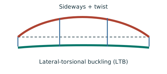
- Divide the beam at effective lateral restraints.
- Use each segment’s effective length to obtain its buckling resistance.
- Compare that resistance with the segment’s equivalent moment demand.
Remember: A section bending check alone does not check lateral-torsional buckling.
The in the last term is intentional: source Eq.8.81 has barred, first-order Mᵧ. The Mᴸᵀ is already amplified. All three interactions pass; flexural member interaction is closest to .
Animation labA strong slice can belong to an unstable member
Supplement to the original lesson. Enable JavaScript to play, step through calculations and rotate 3D models. The following explanation remains readable offline.
- Combine axial compression and the two bending demands using the specified section resistances.
- The whole member adds effective-length and buckling-curve effects.
- This uses its own moment factor and bending resistance; it is not a copy of the section check.
- Elastic, plastic and buckling resistances are not interchangeable. Read the three original expressions and their first-order/amplified moments.
Compact exam answer
S355 UC: , Class 1. Section utilisation . ; , ; curves b/c give , . . , ; elastic resistance /; flexural-buckling utilisation . , , , , ; axial force/LTB utilisation . All pass.
Mistakes to avoid
- Use , not , for the flange.
- Apply the 1.2pᵧZ ceiling on the minor axis.
- Do not use capped plastic capacities in the member interaction.
- Distinguish applied end signs from internal moment-diagram signs.
- Keep first-order Mᵧ in the source Eq.8.81 term.
Procedure for an unfamiliar variant
- Identify axial load, any moments, actual length and restraints in each axis.
- Choose/read a section and confirm strength from the actual thickness.
- Check the appropriate flange and web local-slenderness limits.
- Find and separately; select each axis curve and interpolate .
- Calculate both axial resistances and identify the governing axis.
- If moments exist, complete section, flexural and axial/LTB interactions using their own capacities and moment definitions.
Independent self-check
Try it yourself. Invented variant: only the imposed major-axis end moments in the given factored schedule are replaced by/; treat these as a increase of the stated total first-order moments, with axial load and moments unchanged. How do the checks change?
Reveal answer and reasoning
-axis end-moment ratio remains , so , are unchanged.. Section utilisation increases by to . Flexural-buckling utilisation increases by to . LTB utilisation increases by to . All still pass, with resistance properties unchanged.
Animation labA strong slice can belong to an unstable member
Supplement to the original lesson. Enable JavaScript to play, step through calculations and rotate 3D models. The following explanation remains readable offline.
- Combine axial compression and the two bending demands using the specified section resistances.
- The whole member adds effective-length and buckling-curve effects.
- This uses its own moment factor and bending resistance; it is not a copy of the section check.
- Elastic, plastic and buckling resistances are not interchangeable. Read the three original expressions and their first-order/amplified moments.
Animation labRead the moment shape within one segment
Supplement to the original lesson. Enable JavaScript to play, step through calculations and rotate 3D models. The following explanation remains readable offline.
- Moment ordinates must belong to the same effective unbraced segment.
- Same-side and reverse-curvature diagrams have different signed end ratios.
- The markers show ¼, ½ and ¾ of this segment, not of the entire beam.
- LTB and column flexural factors are different. Preserve their individual bounds and coefficient sets.
8. Simple construction: eccentric reactions still bend columns
Simple explanation: A pinned beam can still bend its column
Its reaction can miss the column centre and create a lever arm.
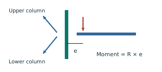
- Find the reaction’s actual nominal eccentricity.
- Multiply reaction by eccentricity to obtain the joint moment.
- Share that moment using the stated column-stiffness model.
Remember: Equal sharing needs equal relevant stiffness; it is not automatic.
A simply supported beam-to-column joint does not transmit a rigid-frame end moment, but its vertical reaction may act away from the column centre. The nominal eccentricity is measured from the column centroid to the reaction line. For a beam resting on a column face, take the reaction position as the larger of from that face and the centre of stiff bearing. Add the centroid-to-face distance (for the illustrated major-axis case, ).
For identical sections above and below, cancels. A3 m lower column is twice as stiff by as a upper one, so shares are and . Opposite equal reactions cancel their nominal moments about that axis but still add to axial compression. The upper column carries roof loads; the lower carries roof plus intermediate-floor loads. Do not distribute accumulated axial load using the moment-stiffness fractions.
The source allows all beams fully loaded without pattern loading for this simplified column procedure. It also says a beam loaded above of its capacity should not be assumed to afford column rotational restraint. These are applicability conditions, not universal properties of every beam connection. The special 0.5L/rᵧ rule uses actual , not the reduced effective column length.
Column example 3: loads and eccentric moments in two storeys
Open this example on its own page
Check UC S355 in a two-storey simple-construction column. The lower storey is , the upper . Use the supplied reaction table and stated construction assumptions, including a pinned base and moment amplification.
Original source: LectureNotes/Ch 4_Column.pdf — p. 25, p. 26, p. 27, p. 28, p. 29, p. 30, p. 31. Values tagged given are in the question or diagram; lookup values come from a named table; calculated values follow from the working; assumptions are stated explicitly.
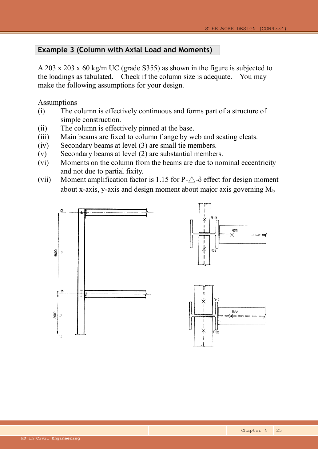
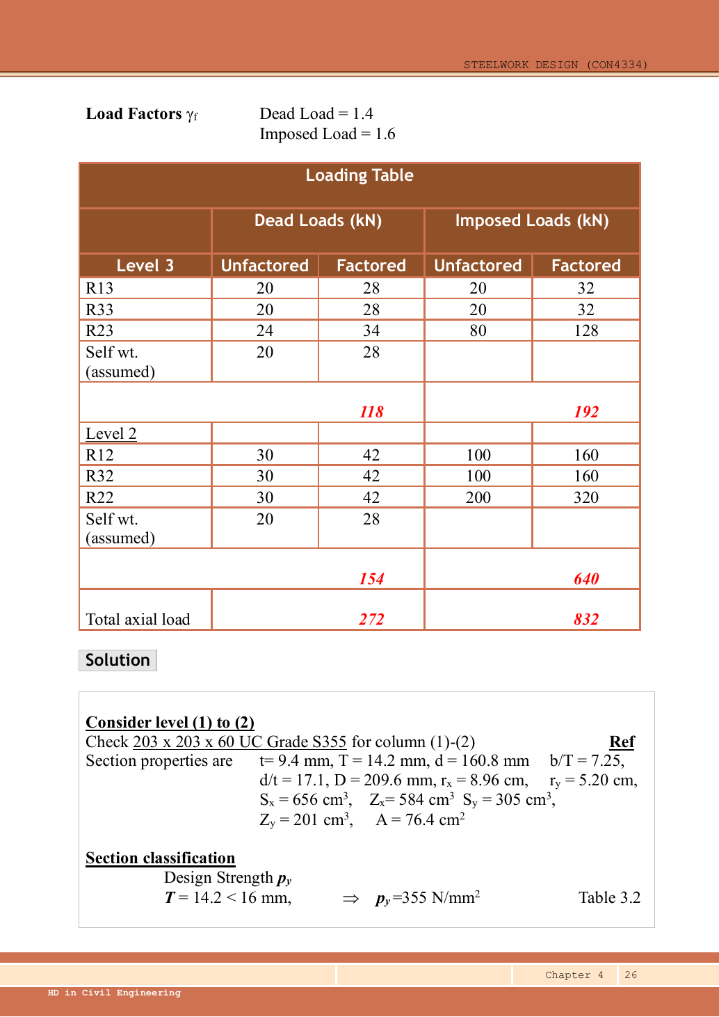
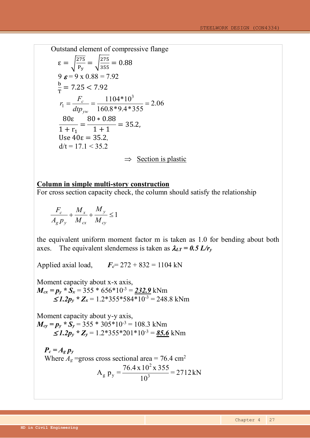
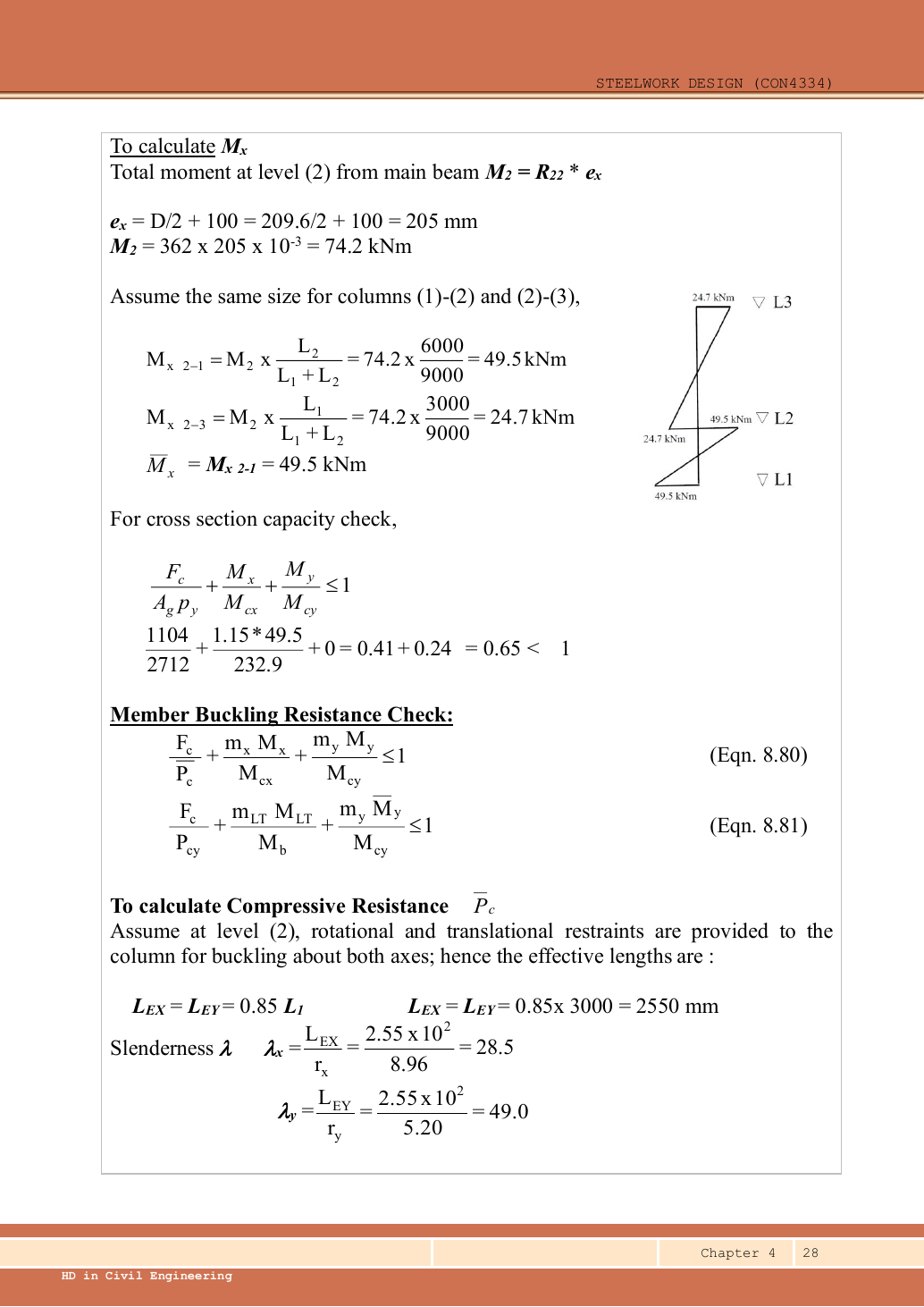
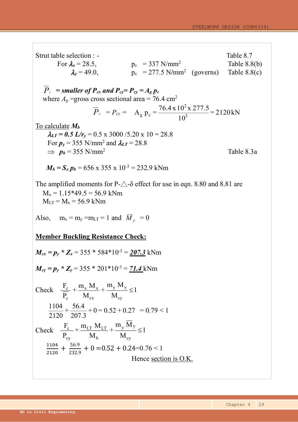
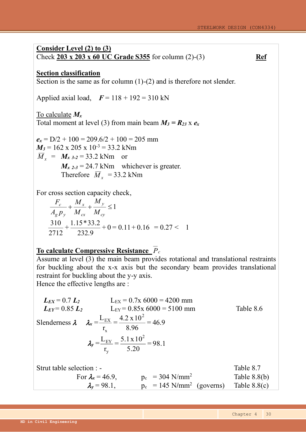
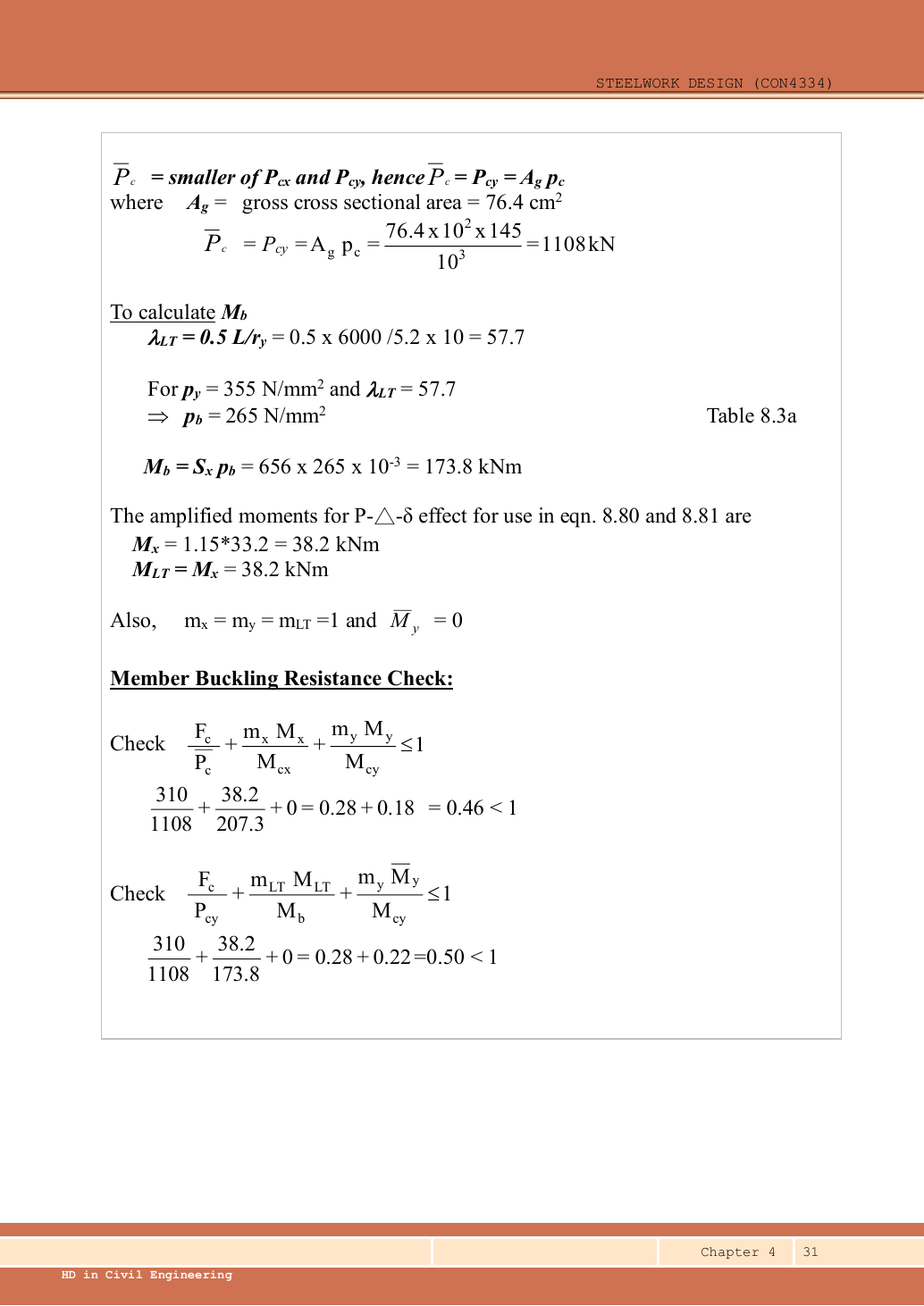
Read the diagram and collect the data
| Given model | Implication |
|---|---|
| Continuous column, simple beam construction | Use nominal eccentricity and moment sharing; all moment factors are . |
| Base effectively pinned | Lower segment has no base rotational fixity. Substantial level 2 members give the source’s upper restraint assumption. |
| Roof secondary beams are small ties | Provide positional but not rotational restraint for the upper column’s weak-axis buckling. |
| Main beams connect by web and seating cleats | Source adopts reaction line beyond the column face. |
| Self-weight | Source assumes characteristic dead self-weight at each level; include it once per level. |
| Section data | Data p.11: , , , , , , , , , , , , . |
Before calculating: recognition and strategy
There are two separate accounting tasks. Axial load accumulates down the column. Eccentric reactions create a net joint moment which is shared between the upper and lower column in proportion to . Equal opposite secondary reactions cancel their moments, but their vertical loads still add. Keep these operations separate. This solution retains arithmetic precision; a short comparison also explains the source’s rounded values.
1. Recalculate every reaction-table entry and storey total
| Level/reaction | Given () | Given () | Ultimate total | ||
|---|---|---|---|---|---|
| 3: | |||||
| 3: | |||||
| 3: | |||||
| 3: assumed self-weight | |||||
| 3 totals | |||||
| 2: | |||||
| 2: | |||||
| 2: | |||||
| 2: assumed self-weight | |||||
| 2 added totals |
Animation labFrom characteristic to design load
Supplement to the original lesson. Enable JavaScript to play, step through calculations and rotate 3D models. The following explanation remains readable offline.
- G is permanent load; Q is imposed load. A surface load and a line load also have different units.
- This illustration uses the course gravity case . Other combinations in the original text retain their own factors.
- For illustrative , change Q and watch each separate contribution.
- Do not carry this ULS total automatically into deflection. Follow the stated SLS load case.
2. Strength and section classification
The lower section’s larger axial compression is sufficient for checking this section’s worst compression/bending web limit. The selected section has the same geometry throughout both storeys.
Animation labWhy thin elements buckle locally
Supplement to the original lesson. Enable JavaScript to play, step through calculations and rotate 3D models. The following explanation remains readable offline.
- The flange outstand and web have different widths, thicknesses and edge support conditions.
- A thinner plate can wrinkle locally before the complete member loses stability.
- Class 1 allows plastic rotation; Class 2 reaches plastic resistance; Class 3 reaches elastic resistance; Class 4 requires effective properties.
- Check every relevant compression element with the supplied limits and stress distribution. The deformation shown is qualitative.
3. Calculate section and elastic member capacities
The linear section interaction uses and . The member interaction uses and . The source reuses similar notation for different definitions; keep a clearly labelled capacity list.
Animation labCompression and tension across a section
Supplement to the original lesson. Enable JavaScript to play, step through calculations and rotate 3D models. The following explanation remains readable offline.
- For sagging, the top flange is in compression and the bottom in tension; hogging reverses this.
- Elastic bending stress varies with distance from the neutral axis: .
- The section class governs whether elastic, plastic or effective properties may be used.
- Use the shear at the section under examination; the largest shear elsewhere is not automatically coexistent.
4. Nominal eccentricity and stiffness sharing at level 2
Simple explanation: A pinned beam can still bend its column
Its reaction can miss the column centre and create a lever arm.
- Find the reaction’s actual nominal eccentricity.
- Multiply reaction by eccentricity to obtain the joint moment.
- Share that moment using the stated column-stiffness model.
Remember: Equal sharing needs equal relevant stiffness; it is not automatic.
The main beam reaction acts on one flange. takes us from the centroid to the flange face; the nominal then takes us to the source’s reaction line. and have equal magnitudes on opposite sides, so their minor-axis nominal moments cancel.
The lower storey is shorter, hence stiffer and receives the larger moment share. The source rounds to , to and shares to /. The little moment diagrams on p.28 show the moment components associated with this joint sharing; they are not additional applied point loads.
Animation labEccentric reactions and stiffness sharing
Supplement to the original lesson. Enable JavaScript to play, step through calculations and rotate 3D models. The following explanation remains readable offline.
- A beam reaction can act away from the column centre even at a nominally pinned beam connection.
- . Opposing reactions can cancel part of the signed moment, while both still add compression.
- The course simple model distributes the joint moment in proportion to of the columns above and below.
- Equal relevant stiffness gives half each. A roof joint with no upper column is a different case.
5. Lower-storey section interaction
Simple explanation: The column needs more than one pass
A slice can be strong while the whole member still buckles.
- Check cross-section compression plus bending.
- Then check the separate member-buckling expressions.
- Keep each moment, factor and resistance in its specified expression.
Remember: The three checks do not share interchangeable denominators.
Using the rounded source loads and moments gives . Both precision levels agree with the source result of approximately .
Animation labA strong slice can belong to an unstable member
Supplement to the original lesson. Enable JavaScript to play, step through calculations and rotate 3D models. The following explanation remains readable offline.
- Combine axial compression and the two bending demands using the specified section resistances.
- The whole member adds effective-length and buckling-curve effects.
- This uses its own moment factor and bending resistance; it is not a copy of the section check.
- Elastic, plastic and buckling resistances are not interchangeable. Read the three original expressions and their first-order/amplified moments.
6. Lower-storey member buckling
Simple explanation: Why a long column can fail before crushing
Push a long thin ruler from both ends: it may bow sideways first.
- Find effective length and radius of gyration for each axis.
- Calculate slenderness for both directions.
- Use the appropriate buckling curve before forming resistance.
Remember: Compare the final resistances; slenderness alone may not identify the controlling axis.
The source assumes rotational and positional restraint at level 2 in both axes; the base is pinned. Table 8.6 recommended fixed/pinned factor is . Use that assumed model explicitly, rather than inferring a rigid base from the drawing’s plate line.
Simple construction sets all factors to . For bending buckling use actual storey length , not :
Animation labA strong slice can belong to an unstable member
Supplement to the original lesson. Enable JavaScript to play, step through calculations and rotate 3D models. The following explanation remains readable offline.
- Combine axial compression and the two bending demands using the specified section resistances.
- The whole member adds effective-length and buckling-curve effects.
- This uses its own moment factor and bending resistance; it is not a copy of the section check.
- Elastic, plastic and buckling resistances are not interchangeable. Read the three original expressions and their first-order/amplified moments.
7. Upper-storey governing moment and section interaction
The upper-storey moment is governed by the roof reaction, not automatically the moment inherited at level 2. The source uses , giving amplified . Its printed comes from early rounding of the separate utilisation terms; full arithmetic is about at two decimal places.
Animation labA strong slice can belong to an unstable member
Supplement to the original lesson. Enable JavaScript to play, step through calculations and rotate 3D models. The following explanation remains readable offline.
- Combine axial compression and the two bending demands using the specified section resistances.
- The whole member adds effective-length and buckling-curve effects.
- This uses its own moment factor and bending resistance; it is not a copy of the section check.
- Elastic, plastic and buckling resistances are not interchangeable. Read the three original expressions and their first-order/amplified moments.
8. Upper-storey buckling about both axes
The main roof beam supplies the source’s major-axis rotational restraint. The small secondary roof ties only restrain position in the weak direction. With level 2 restrained, the lecture uses for and for .
Both storeys pass all three demonstrated interaction checks. The lower-storey flexural interaction, approximately , is the largest. The original source-rounded results are approximately lower // and upper //.
Animation labA strong slice can belong to an unstable member
Supplement to the original lesson. Enable JavaScript to play, step through calculations and rotate 3D models. The following explanation remains readable offline.
- Combine axial compression and the two bending demands using the specified section resistances.
- The whole member adds effective-length and buckling-curve effects.
- This uses its own moment factor and bending resistance; it is not a copy of the section check.
- Elastic, plastic and buckling resistances are not interchangeable. Read the three original expressions and their first-order/amplified moments.
Compact exam answer
Using exact arithmetic: upper/lower compression /. pᵧ355,Class 1; A𝗀pᵧ2,712.2 kN; section capacities /; elastic /. ; level 2 moment shares /. Amplified lower moment ; upper governing . Lower ,Mᵦ232.88; interactions //. Upper ,Mᵦ173.7391; interactions //. Both storeys adequate under the stated simple-construction restraint assumptions.
Mistakes to avoid
- Accumulate both levels for lower axial load.
- Cancel opposite moments, not the underlying compressive reactions.
- Share moment by , not equally and not by axial-force ratios.
- Use actual storey length in 0.5L/rᵧ.
- Do not treat a small roof tie as rotational restraint.
Procedure for an unfamiliar variant
- Trace the loads above each column segment and keep dead/imposed components separate.
- Read actual storey heights, section properties and end restraints in both axes.
- For simple construction derive nominal eccentric moments and share them by .
- Classify the section and form the correct section and member resistances.
- Apply only the prescribed load reductions and moment amplification rules.
- Check every storey segment and report both the governing check and source assumptions.
Independent self-check
Try it yourself. Invented variant: change only the upper-storey length from to , retaining the same column section and level 2 moment . How is that joint moment shared?
Reveal answer and reasoning
The upper and lower values now match, so each receives . The lower amplified share becomes . This redistribution does not alter the accumulated axial loads. Upper buckling lengths and 0.5L/rᵧ also change and must be recalculated; the original upper resistance cannot be reused.
Animation labEccentric reactions and stiffness sharing
Supplement to the original lesson. Enable JavaScript to play, step through calculations and rotate 3D models. The following explanation remains readable offline.
- A beam reaction can act away from the column centre even at a nominally pinned beam connection.
- . Opposing reactions can cancel part of the signed moment, while both still add compression.
- The course simple model distributes the joint moment in proportion to of the columns above and below.
- Equal relevant stiffness gives half each. A roof joint with no upper column is a different case.
Column example 4: tributary area and cumulative column loads
Open this example on its own page
Design internal column A in S355 for axial load only. Roof dead/imposed intensities are /; floor intensities /. Upper storey height ; lower . The foundation is fixed. Floor beams prevent translation but do not restrain column rotation. All given dead loads include beam and column self-weight.
Original source: LectureNotes/Ch 4_Column.pdf — p. 32, p. 33, p. 34, p. 35. Values tagged given are in the question or diagram; lookup values come from a named table; calculated values follow from the working; assumptions are stated explicitly.
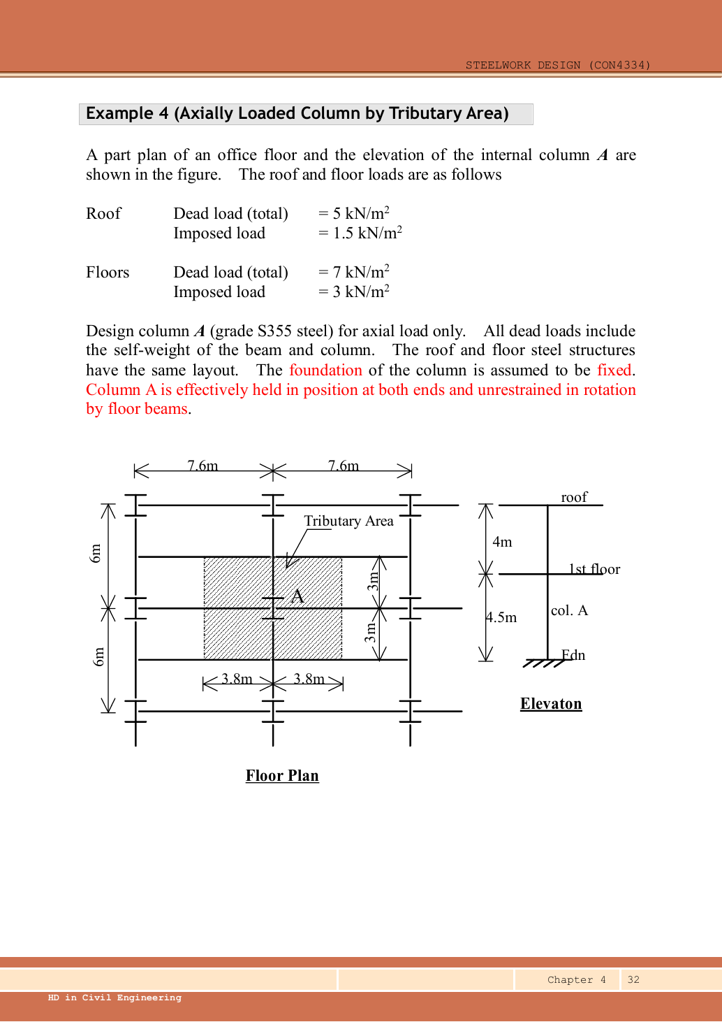
Read the diagram and collect the data
| Input | Where to read it |
|---|---|
| Tributary dimensions | Plan labels and ; use plan area, not storey height. |
| Vertical dimensions | Elevation upper and lower. |
| Roof/floor loads | Question text; the same floor plan applies at both levels. |
| Axial-only scope | Explicitly requested; no eccentric moment is introduced into this exercise. |
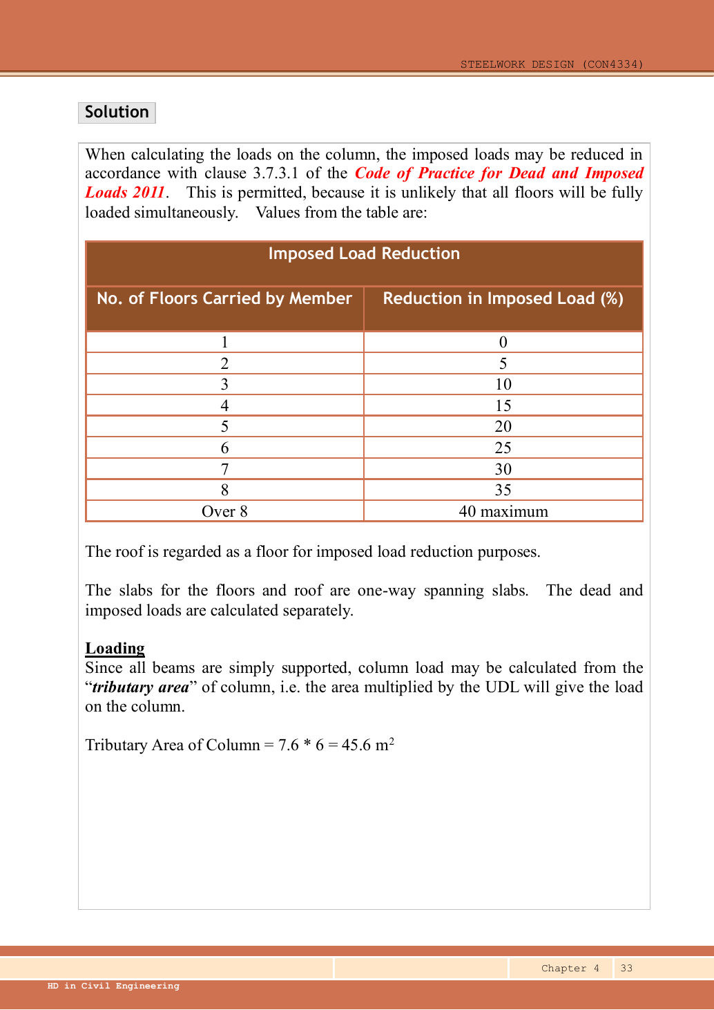
| Imposed reduction | Lecture p.33 applies its 2011 load-code floor-count table; roof counts as a floor. |
Before calculating: recognition and strategy
Multiply each level’s pressure by the area feeding the column. The upper segment carries only roof loading; the lower carries roof plus first floor. Reduce the cumulative imposed load only when the source’s permitted floor-count rule applies. After factoring, design each storey separately because loads, lengths and end conditions differ.
1. Derive the tributary area from the hatched plan
Simple explanation: How a floor load reaches a beam
Each beam collects the load from its own strip of floor.
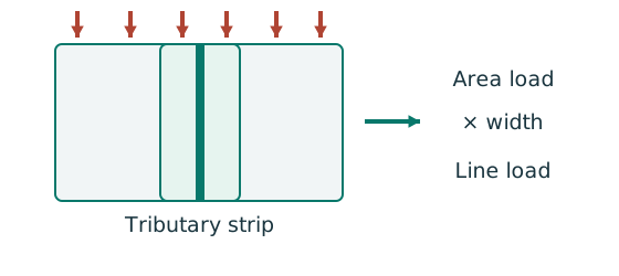
- Find the tributary width from the actual plan.
- Area load × tributary width gives load per beam length.
- A supporting beam receives the other beam’s end reaction.
Remember: A reaction becomes a point load, not automatically a UDL.
Half of each adjacent simply supported bay reaches column A. The hatch is a load-allocation area, not the column’s steel cross-sectional area. Both roof and floor use .
Animation labFollow the floor load in 3D
Supplement to the original lesson. Enable JavaScript to play, step through calculations and rotate 3D models. The following explanation remains readable offline.
- The floor carries pressure in . The highlighted strip belongs to one secondary beam.
- Multiply pressure by tributary width: . The illustration uses .
- A primary beam receives the secondary beam reaction at their connection, not a new full-span UDL.
- Trace reactions down to columns and foundations. Count each loaded area once.
2. Read the source’s floor-count reduction
| Floors carried | Over | ||||||||
|---|---|---|---|---|---|---|---|---|---|
| Imposed reduction | maximum |
The upper member supports one roof level → reduction. The lower supports roof plus first floor →two levels →. Retain of the cumulative imposed load below the floor. This is the rule applied by this lecture example, attributed there to the 2011 Dead and Imposed Loads Code; do not extend it automatically to an occupancy or question where reduction is disallowed. Dead load is not reduced.
Animation labFollow the floor load in 3D
Supplement to the original lesson. Enable JavaScript to play, step through calculations and rotate 3D models. The following explanation remains readable offline.
- The floor carries pressure in . The highlighted strip belongs to one secondary beam.
- Multiply pressure by tributary width: . The illustration uses .
- A primary beam receives the secondary beam reaction at their connection, not a new full-span UDL.
- Trace reactions down to columns and foundations. Count each loaded area once.
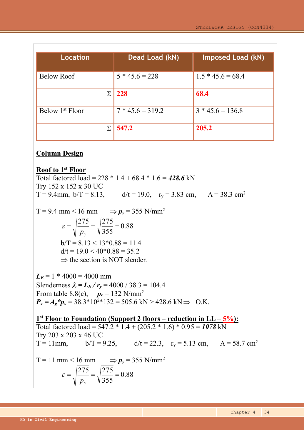
3. Compute characteristic and ultimate loads at each level
All self-weight is already included. The lower load uses the whole accumulated load rather than adding an already factored/reduced upper force to a separately reduced floor force.
Animation labFrom characteristic to design load
Supplement to the original lesson. Enable JavaScript to play, step through calculations and rotate 3D models. The following explanation remains readable offline.
- G is permanent load; Q is imposed load. A surface load and a line load also have different units.
- This illustration uses the course gravity case . Other combinations in the original text retain their own factors.
- For illustrative , change Q and watch each separate contribution.
- Do not carry this ULS total automatically into deflection. Follow the stated SLS load case.
4. Select and check the upper column
Simple explanation: A pinned beam can still bend its column
Its reaction can miss the column centre and create a lever arm.
- Find the reaction’s actual nominal eccentricity.
- Multiply reaction by eccentricity to obtain the joint moment.
- Share that moment using the stated column-stiffness model.
Remember: Equal sharing needs equal relevant stiffness; it is not automatic.
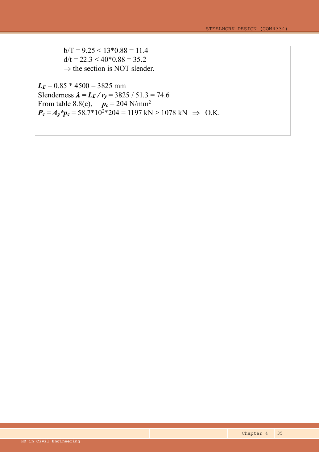
Trial UC. Data File p.11 gives , , , , , . The original lecture uses the same area . , giving . Both ends are held in position but free to rotate, so , with both axes having .
The source uses rounded , so and prints . Exact interpolation gives ; both pass. The previously omitted major-axis comparison is provided above.
Animation labEffective length and buckling axes
Supplement to the original lesson. Enable JavaScript to play, step through calculations and rotate 3D models. The following explanation remains readable offline.
- A column can bow sideways before its section reaches the crushing resistance.
- Each axis has its own radius of gyration and restraint spacing.
- , with compatible length units. A tie affects only the directions it actually restrains.
- Select each buckling curve and compressive strength before forming Pc. The governing axis is determined by resistance, not slenderness alone.
5. Select and check the lower column
Simple explanation: The column needs more than one pass
A slice can be strong while the whole member still buckles.
- Check cross-section compression plus bending.
- Then check the separate member-buckling expressions.
- Keep each moment, factor and resistance in its specified expression.
Remember: The three checks do not share interchangeable denominators.
Trial UC. Data File p.11 gives , , , , , . The flange thickness again gives . The base is fixed; the floor end is held in position but free to rotate, so use the recommended factor .
The source rounds to , giving (printed ). Exact interpolation gives . Both selected columns pass the requested axial-only design; the lower weak-axis check is more highly utilised.
Animation labEffective length and buckling axes
Supplement to the original lesson. Enable JavaScript to play, step through calculations and rotate 3D models. The following explanation remains readable offline.
- A column can bow sideways before its section reaches the crushing resistance.
- Each axis has its own radius of gyration and restraint spacing.
- , with compatible length units. A tie affects only the directions it actually restrains.
- Select each buckling curve and compressive strength before forming Pc. The governing axis is determined by resistance, not slenderness alone.
Compact exam answer
. Roof / is /; lower-storey accumulation /. Upper-storey ultimate force ; lower-storey imposed load after reduction gives . Upper-storey UC: non-slender, , . Lower-storey UC: non-slender, , . Both are S355 with , governed by minor-axis curve c; both are adequate.
Mistakes to avoid
- Do not use or elevation heights when calculating tributary plan area.
- Include roof load in the lower segment.
- Reduce only imposed load and count the roof as instructed.
- Do not add self-weight twice.
- Use fixed/pinned recommended for the lower column, not the upper one.
Procedure for an unfamiliar variant
- Trace the loads above each column segment and keep dead/imposed components separate.
- Read actual storey heights, section properties and end restraints in both axes.
- For simple construction derive nominal eccentric moments and share them by .
- Classify the section and form the correct section and member resistances.
- Apply only the prescribed load reductions and moment amplification rules.
- Check every storey segment and report both the governing check and source assumptions.
Independent self-check
Try it yourself. Invented variant: imposed-load reduction is explicitly prohibited. Does the selected lower column still pass?
Reveal answer and reasoning
Lower force becomes . Compare with : utilisation, so it still passes. The roof segment is unchanged because it already had zero reduction.
Animation labEffective length and buckling axes
Supplement to the original lesson. Enable JavaScript to play, step through calculations and rotate 3D models. The following explanation remains readable offline.
- A column can bow sideways before its section reaches the crushing resistance.
- Each axis has its own radius of gyration and restraint spacing.
- , with compatible length units. A tie affects only the directions it actually restrains.
- Select each buckling curve and compressive strength before forming Pc. The governing axis is determined by resistance, not slenderness alone.
Animation labEccentric reactions and stiffness sharing
Supplement to the original lesson. Enable JavaScript to play, step through calculations and rotate 3D models. The following explanation remains readable offline.
- A beam reaction can act away from the column centre even at a nominally pinned beam connection.
- . Opposing reactions can cancel part of the signed moment, while both still add compression.
- The course simple model distributes the joint moment in proportion to of the columns above and below.
- Equal relevant stiffness gives half each. A roof joint with no upper column is a different case.
9. A repeatable exam sequence
- Identify simple or continuous construction, sway status, column segment, effective lengths in both axes, section and grade.
- Assemble factored axial load at each level; derive any eccentric moments or read given end moments.
- Read exact section properties and thickness-dependent pᵧ. Classify local elements under the applicable stress pattern.
- Compute capped section moment resistances and check the axial/biaxial section interaction.
- Calculate and , choose the proper curves, interpolate and form both axis resistances.
- For continuous construction obtain , and mᴸᵀ from their separate tables. For simple construction set all three to .
- Use the correct amplified/first-order moments and elastic pᵧZ denominators for flexural interaction.
- Compute λᴸᵀ using the appropriate simple/continuous rule; read pᵦ, calculate Mᵦ and check Eq.8.81.
- State all utilisation ratios and whether every required check is.
Animation labEffective length and buckling axes
Supplement to the original lesson. Enable JavaScript to play, step through calculations and rotate 3D models. The following explanation remains readable offline.
- A column can bow sideways before its section reaches the crushing resistance.
- Each axis has its own radius of gyration and restraint spacing.
- , with compatible length units. A tie affects only the directions it actually restrains.
- Select each buckling curve and compressive strength before forming Pc. The governing axis is determined by resistance, not slenderness alone.
Practise this chapter: tutorials, assignments and past-paper answers →