Column example 4: tributary area and cumulative column loads
← Read this lecture example beside its chapter concepts
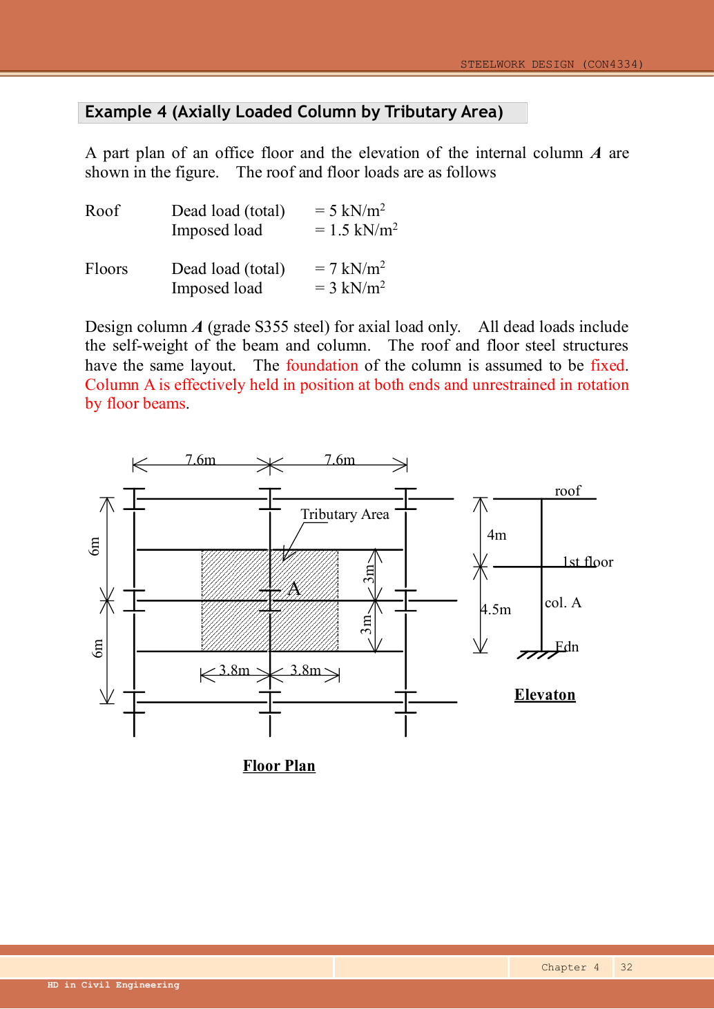
Design internal column A in S355 for axial load only. Roof dead/imposed intensities are /; floor intensities /. Upper storey height ; lower . The foundation is fixed. Floor beams prevent translation but do not restrain column rotation. All given dead loads include beam and column self-weight.
Original source: LectureNotes/Ch 4_Column.pdf — p. 32, p. 33, p. 34, p. 35.
A given value comes from the question or diagram.
A lookup value comes from the named table.
A calculated value follows from the working.
Each assumption is stated where the calculation needs it.
Known information, diagram labels and unknowns
Follow one strip of floor
An area load must become a beam load before beam reactions can be calculated.
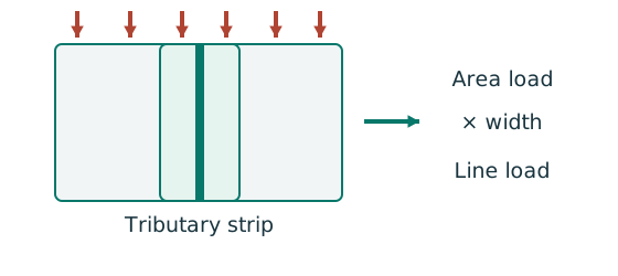
Prediction, then explanation. At fixed area load, twice the tributary width gives twice the line load. An end reaction remains a concentrated force.
Consider one metre along the beam. The associated floor area is b square metres. Multiply area load by that width.
q is area load in kN/m²; b is tributary width in m; w is line load in kN/m.
Scope. Determine b from slab spanning and supports. Add beam self-weight separately. A secondary-beam reaction is not automatically a UDL.
Check and takeaway. Illustration: . The width cancels one length unit.
A table value has conditions
Find a design property without mixing a row, column or standard from a different case.
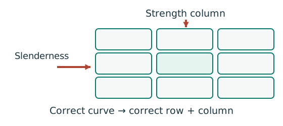
Prediction, then explanation. A different flange thickness can select a lower design strength even when the steel grade name remains unchanged.
Match the complete section designation. Read the relevant axis and unit. For strength tables, select material, thickness and curve before interpolating.
Given values come from the question. Lookup values come from a named table. Assumed values require an explicit condition.
Scope. A missing row or omitted restraint cannot be recovered from a schematic’s scale. Keep the result conditional when required data are absent.
Check and takeaway. Record the table, row, column and unit beside the substitution. That makes a later check possible.
Apply the reasoning to this section’s data and conditions
| Input | Where to read it |
|---|---|
| Tributary dimensions | Plan labels and . Use plan area, not storey height. |
| Vertical dimensions | Elevation upper and lower. |
| Roof/floor loads | Question text. The same floor plan applies at both levels. |
| Axial-only scope | Explicitly requested. No eccentric moment is introduced into this exercise. |
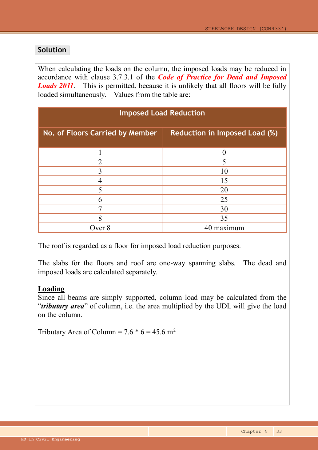
| Imposed reduction | Lecture p.33 applies its 2011 load-code floor-count table; roof counts as a floor. |
Why this method applies
Use the same mechanism: Follow one strip of floor. At fixed area load, twice the tributary width gives twice the line load. An end reaction remains a concentrated force.
Apply the reasoning to this section’s data and conditions
Multiply each level’s pressure by the area feeding the column.
The upper segment carries only roof loading.
The lower carries roof plus first floor.
Reduce the cumulative imposed load only when the source’s permitted floor-count rule applies.
After factoring, design each storey separately because loads, lengths and end conditions differ.
1. Derive the tributary area from the hatched plan
Use the same mechanism: Follow one strip of floor. At fixed area load, twice the tributary width gives twice the line load. An end reaction remains a concentrated force.
Apply the reasoning to this section’s data and conditions
Physical interpretation: How a floor load reaches a beam
Each beam collects the load from its own strip of floor.
Sketch, not to scale; use the original dimensions.
- Find the tributary width from the actual plan.
- Area load × tributary width gives load per beam length.
- A supporting beam receives the other beam’s end reaction.
Remember: A reaction becomes a point load, not automatically a UDL.
Half of each adjacent simply supported bay reaches column A.
The hatch is a load-allocation area, not the column’s steel cross-sectional area.
Both roof and floor use .
Mechanism detailsFollow the floor load in 3D
The complete mechanism is explained below.
Read each stage together with its stated conditions; playback and interaction are not required.
The floor carries pressure in .
The highlighted strip belongs to one secondary beam.
Multiply pressure by tributary width: .
The illustration uses .
- A primary beam receives the secondary beam reaction at their connection, not a new full-span UDL.
Trace reactions down to columns and foundations.
Count each loaded area once.
2. Read the source’s floor-count reduction
Use the same mechanism: Follow one strip of floor. At fixed area load, twice the tributary width gives twice the line load. An end reaction remains a concentrated force.
Keep load categories separate
A floor carries permanent material and changing occupancy loads. Find the design load for the stated check.
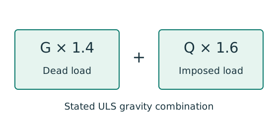
Prediction, then explanation. Increasing imposed load changes its own term. It does not change the dead-load factor or the steel stiffness.
First convert mass to weight where required. Next collect G and Q in compatible units. Apply the combination specified by the course problem.
G is characteristic dead load; Q is characteristic imposed load. Wu is the design load for this course gravity combination.
Scope. This combination is not universal. Use the specified service load for deflection and the stated factors for other standards or cases.
Check and takeaway. Illustration: G = 10 kN and Q = 5 kN give 22 kN. Factoring their sum by one guessed factor loses the distinction.
Use the same mechanism: A table value has conditions. A different flange thickness can select a lower design strength even when the steel grade name remains unchanged.
Apply the reasoning to this section’s data and conditions
| Floors carried | Over | ||||||||
|---|---|---|---|---|---|---|---|---|---|
| Imposed reduction | maximum |
The upper member supports one roof level → reduction.
The lower supports roof plus first floor →two levels →.
Retain of the cumulative imposed load below the floor.
This is the rule applied by this lecture example, attributed there to the 2011 Dead and Imposed Loads Code.
Do not extend it automatically to an occupancy or question where reduction is disallowed.
Dead load is not reduced.
Mechanism detailsFollow the floor load in 3D
The complete mechanism is explained below.
Read each stage together with its stated conditions; playback and interaction are not required.
The floor carries pressure in .
The highlighted strip belongs to one secondary beam.
Multiply pressure by tributary width: .
The illustration uses .
- A primary beam receives the secondary beam reaction at their connection, not a new full-span UDL.
Trace reactions down to columns and foundations.
Count each loaded area once.
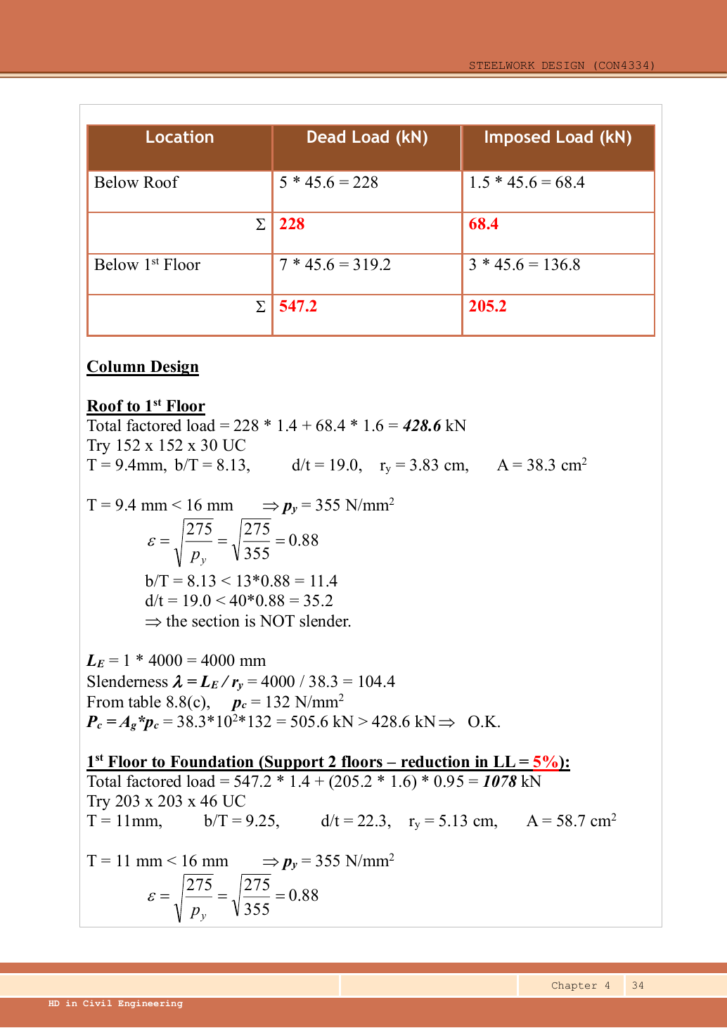
3. Compute characteristic and ultimate loads at each level
Use the same mechanism: Keep load categories separate. Increasing imposed load changes its own term. It does not change the dead-load factor or the steel stiffness.
Apply the reasoning to this section’s data and conditions
All self-weight is already included.
The lower load uses the whole accumulated load rather than adding an already factored/reduced upper force to a separately reduced floor force.
Mechanism detailsFrom characteristic to design load
The complete mechanism is explained below.
Read each stage together with its stated conditions; playback and interaction are not required.
G is permanent load; Q is imposed load.
A surface load and a line load also have different units.
This illustration uses the course gravity case .
Other combinations in the original text retain their own factors.
- For illustrative , the separate load contributions show what changes when Q increases.
Do not carry this ULS total automatically into deflection.
Follow the stated SLS load case.
4. Select and check the upper column
Check buckling about both axes
Determine which buckling direction limits the compressed member.
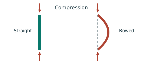
Prediction, then explanation. At fixed radius, longer effective length raises slenderness. The supplied buckling curve generally gives lower compressive strength.
Calculate slenderness about each axis. Select each axis’s curve from section type and thickness. Then obtain and compare the two compressive resistances.
Effective lengths and radii use mm. pc is compressive strength in N/mm²; Ag is gross area in mm²; Pc is in N.
Scope. Do not select the governing axis using radius alone. Effective length and buckling curve can differ. A combined column also needs interaction checks.
Check and takeaway. A short-section yield resistance is not the same as long-member buckling resistance. Keep py and pc distinct.
Find which plate buckles first
Before using plastic bending resistance, check whether the flange and web can sustain the required stress distribution.
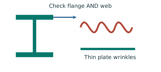
Prediction, then explanation. At fixed width, a thinner plate has a larger width-to-thickness ratio. Local buckling then becomes more restrictive.
Calculate the flange and web ratios separately. Compare each with the limits for its stress condition. The worse class governs.
py is the design yield strength in N/mm². ε is a dimensionless scale used in the supplied classification limits.
Scope. Pure bending and uniform compression use different web limits. Class 2 allows plastic resistance but not the Class 1 rotation capability.
Check and takeaway. A Class 1 web and Class 2 flange give a Class 2 section. Do not average the class numbers.
Use the same mechanism: A table value has conditions. A different flange thickness can select a lower design strength even when the steel grade name remains unchanged.
Apply the reasoning to this section’s data and conditions
Physical interpretation: A pinned beam can still bend its column
Its reaction can miss the column centre and create a lever arm.
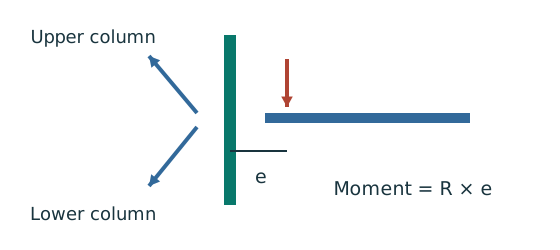
Sketch, not to scale; use the original dimensions.
- Find the reaction’s actual nominal eccentricity.
- Multiply reaction by eccentricity to obtain the joint moment.
- Share that moment using the stated column-stiffness model.
Remember: Equal sharing needs equal relevant stiffness.
It is not automatic.
Trial UC.
Data File p.11 gives , , , , , .
The original lecture uses the same area .
, giving .
Both ends are held in position but free to rotate, so , with both axes having .
The source uses rounded , so and prints .
Exact interpolation gives .
Both pass.
The previously omitted major-axis comparison is provided above.
Mechanism detailsEffective length and buckling axes
The complete mechanism is explained below.
Read each stage together with its stated conditions; playback and interaction are not required.
- A column can bow sideways before its section reaches the crushing resistance.
- Each axis has its own radius of gyration and restraint spacing.
, with compatible length units.
A tie affects only the directions it actually restrains.
Select each buckling curve and compressive strength before forming Pc.
The governing axis is determined by resistance, not slenderness alone.
5. Select and check the lower column
Use the same mechanism: Check buckling about both axes. At fixed radius, longer effective length raises slenderness. The supplied buckling curve generally gives lower compressive strength.
Use the same mechanism: Find which plate buckles first. At fixed width, a thinner plate has a larger width-to-thickness ratio. Local buckling then becomes more restrictive.
Use the same mechanism: A table value has conditions. A different flange thickness can select a lower design strength even when the steel grade name remains unchanged.
Apply the reasoning to this section’s data and conditions
Physical interpretation: The column needs more than one pass
A slice can be strong while the whole member still buckles.
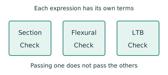
Sketch, not to scale; use the original dimensions.
- Check cross-section compression plus bending.
- Then check the separate member-buckling expressions.
- Keep each moment, factor and resistance in its specified expression.
Remember: The three checks do not share interchangeable denominators.
Trial UC.
Data File p.11 gives , , , , , .
The flange thickness again gives .
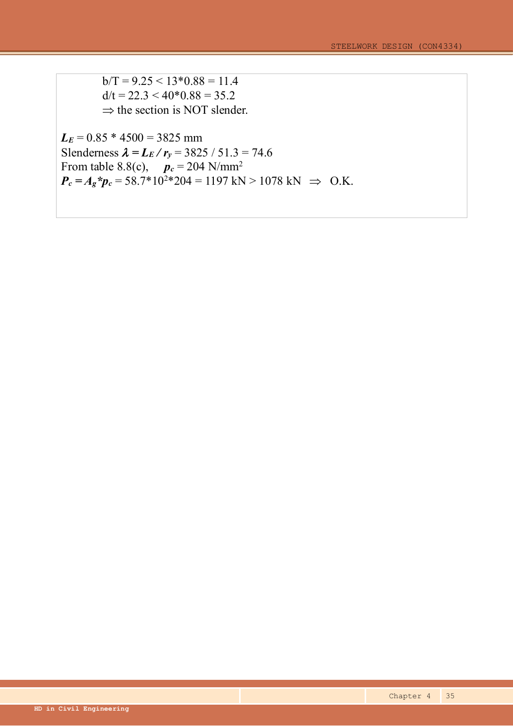
The base is fixed.
The floor end is held in position but free to rotate.
Therefore, use the recommended factor .
The source rounds to , giving (printed ).
Exact interpolation gives .
Both selected columns pass the requested axial-only design.
The lower weak-axis check is more highly utilised.
Mechanism detailsEffective length and buckling axes
The complete mechanism is explained below.
Read each stage together with its stated conditions; playback and interaction are not required.
- A column can bow sideways before its section reaches the crushing resistance.
- Each axis has its own radius of gyration and restraint spacing.
, with compatible length units.
A tie affects only the directions it actually restrains.
Select each buckling curve and compressive strength before forming Pc.
The governing axis is determined by resistance, not slenderness alone.
Result and concise exam wording
A strong cross-section can belong to an unstable member
A column carries axial compression and bending. Explain why more than one check is required.
Prediction, then explanation. At fixed moments and resistances, increasing compression increases utilisation. A section pass cannot remove the length-dependent instability checks.
Separate cross-section, flexural-buckling and LTB interaction equations. Use each equation’s own denominators and first-order or amplified moments.
is a section axial resistance. is a member compression resistance. Elastic and prescribed are different bending denominators.
Scope. Preserve the course barred-moment definitions and Eq. 8.81 convention. Do not substitute plastic moduli into an elastic denominator.
Check and takeaway. Report each requested utilisation and the governing check. The largest properly calculated ratio identifies the closest limit.
Use the same mechanism: Check buckling about both axes. At fixed radius, longer effective length raises slenderness. The supplied buckling curve generally gives lower compressive strength.
Apply the reasoning to this section’s data and conditions
.
Roof / is /; lower-storey accumulation /.
Upper-storey ultimate force ; lower-storey imposed load after reduction gives .
Upper-storey UC: non-slender, , .
Lower-storey UC: non-slender, , .
Both are S355 with , governed by minor-axis curve c.
Both are adequate.
Misconceptions and checks
Use the same mechanism: Follow one strip of floor. At fixed area load, twice the tributary width gives twice the line load. An end reaction remains a concentrated force.
Apply the reasoning to this section’s data and conditions
- Do not use or elevation heights when calculating tributary plan area.
- Include roof load in the lower segment.
- Reduce only imposed load and count the roof as instructed.
- Do not add self-weight twice.
- Use fixed/pinned recommended for the lower column, not the upper one.
How the method transfers to a new variant
Compression acts on the displaced shape
A compressed member moves away from its initial load line. Explain why the bending moment can increase.
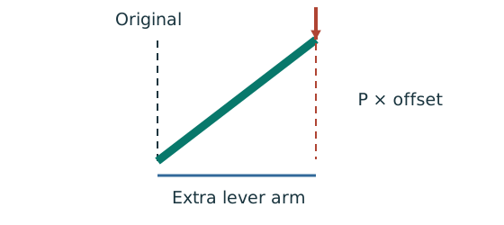
Prediction, then explanation. At fixed axial force, a larger offset creates a larger additional moment. This can further increase the displacement.
Force acting through an offset forms a moment. Second-order analysis includes that changed geometry in equilibrium.
P is axial force. Δ and δ are the relevant perpendicular displacements. Consistent force and length units give moment units.
Scope. Use the amplification or analysis method stated for the frame. Do not amplify an already amplified moment a second time.
Check and takeaway. Zero offset removes this additional moment in the ideal sketch. Real design may still require imperfections and code checks.
An eccentric beam reaction bends the column
A simple beam joint delivers a vertical reaction away from the column centre. Find the resulting column moments.
Prediction, then explanation. Equal opposite-face reactions can cancel a joint moment. Their downward forces still add to column compression.
Sum axial forces first. Calculate the signed eccentric moments. Share the net joint moment between upper and lower columns using the stated stiffness model.
R is reaction; e is perpendicular eccentricity. K denotes the stiffness measure prescribed for moment sharing.
Scope. Equal sharing requires equal stated stiffness. Use actual storey length where the special simple-construction LTB rule requires it.
Check and takeaway. A pin-like beam connection can still cause an eccentric reaction moment in the column. Joint rotation and reaction location are separate facts.
Use the same mechanism: Find which plate buckles first. At fixed width, a thinner plate has a larger width-to-thickness ratio. Local buckling then becomes more restrictive.
Apply the reasoning to this section’s data and conditions
- Trace the loads above each column segment and keep dead/imposed components separate.
- Read actual storey heights, section properties and end restraints in both axes.
- For simple construction derive nominal eccentric moments and share them by .
- Classify the section and form the correct section and member resistances.
- Apply only the prescribed load reductions and moment amplification rules.
- Check every storey segment and report both the governing check and source assumptions.
Prediction with explained answer
Use the same mechanism: A strong cross-section can belong to an unstable member. At fixed moments and resistances, increasing compression increases utilisation. A section pass cannot remove the length-dependent instability checks.
Use the same mechanism: Check buckling about both axes. At fixed radius, longer effective length raises slenderness. The supplied buckling curve generally gives lower compressive strength.
Apply the reasoning to this section’s data and conditions
Prediction and explained answer.
Invented variant: imposed-load reduction is explicitly prohibited.
Does the selected lower column still pass?
Answer and reasoning
Lower force becomes .
Compare with : utilisation, so it still passes.
The roof segment is unchanged because it already had zero reduction.
Mechanism detailsEffective length and buckling axes
The complete mechanism is explained below.
Read each stage together with its stated conditions; playback and interaction are not required.
- A column can bow sideways before its section reaches the crushing resistance.
- Each axis has its own radius of gyration and restraint spacing.
, with compatible length units.
A tie affects only the directions it actually restrains.
Select each buckling curve and compressive strength before forming Pc.
The governing axis is determined by resistance, not slenderness alone.