Column examples: biaxial bending, amplification and interpreting utilisation
This lecture focuses on axial compression with biaxial bending. Read the effective-length, buckling and interaction foundations, then start with complete Example 5. Q2 and Q3 include all three checks; Q5 is slightly above 1 at member level and shows how the lecturer states a marginally OK result.
Abbreviations: DL—Dead Load; LL—Live Load; ULS—Ultimate Limit State; SLS—Serviceability Limit State; UDL—Uniformly Distributed Load; LTB—Lateral-torsional Buckling; UB—Universal Beam; UC—Universal Column.
Key Points
- For axial compression plus biaxial bending, complete the section check followed by both member interaction checks.
- Amplify moments as specified, for example by 1.1 or 1.15, then select governing values.
- Determine from end-moment directions and read , and . These factors apply only to demand terms in member expressions.
- Member denominators use , elastic capacities and , rather than section .
- Compare utilisation with 1. Q5 gives about 1.05, which the lecturer judges marginally OK. Write the values in the answer; do not round to 1.
Key Formulas
Exam Question Types
- Biaxially bent column, Example 5. → Example 5: biaxial checks for a non-sway-frame column (Biaxial Column)
- Eccentric-reaction column and interpreting a result slightly above 1, Q5. → Q5: utilisation slightly above 1, judged marginally OK by the lecturer (Marginal Utilization)
Design flows for these question types
- The approximately 01:30–01:50 break is omitted; assignment-submission matters were also handled during it.
Separate section and member levels in column design (Section versus Member)
What this unit is for: A column carries compression and moments about two axes at once; this unit explains checking the hardest-worked cross-section first, then the whole column against buckling, each with its own capacities.
Picture it this way: Think of the compression and the two moments as three expenses paid from one budget. Each is first written as a fraction of its own limit, and the three fractions together must not pass one whole. For the cross-section the compression limit is ; for the whole column it becomes the smaller .
Prerequisites: Instability can precede material crushing (Buckling) · Combined axial force and bending (Interaction Checks) · Read an I-section and its section table (Section Properties)
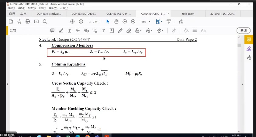
The lecturer restates the two levels. Section expressions assess material and local cross-sectional resistance; member expressions also include length, end restraint and overall instability. Write and separately and note that the former contains no length term.
A column may have different slenderness , buckling curves and end-moment diagrams about and . Keep a separate data column for each. Both being bending directions does not justify a shared factor or modulus.
These are course code methods, not simple addition of three forces. Divide each demand by its resistance to obtain a dimensionless ratio, then compare using the appropriate interaction equation. This structure helps identify incorrect denominators.
Sequence for using column design expressions
Calculate and , obtain from the correct curves, and find . Then handle biaxial moments and LTB according to the problem type.
The section axial-force denominator is ; the member denominator is . The difference represents overall buckling.
Example 5: retain moment signs through all three comparisons (Biaxial Worked Example)
What this unit is for: The moments at the two ends of a column differ in size and direction; this unit keeps their signs and completes three comparisons, one for the cross-section and two for the whole column.
Picture it this way: Bend a long plastic strip with both hands. Turn the ends so it forms one bow, curving to one side; turn them the opposite way and it forms an . The single bow pushes a column towards buckling most, the much less, so the signs of the end moments decide the size of the moment factor.
Prerequisites: Combined axial force and bending (Interaction Checks) · Instability can precede material crushing (Buckling) · Why a beam moves sideways and twists (Lateral-torsional Buckling)
Given end-moment signs follow specified rotations; table follows the bending-diagram convention. The lecturer converts moments +80/+24 to and moments +30/−21 to . Draw end arrows and the internal moment diagram before using the table signs.
Each section capacity takes the smaller candidate; 1.2pyZ governs the weak axis. Member expressions use elastic , plus and moment factors. The three totals differ because their checks differ; do not choose the smallest as the overall conclusion.
The complete example links area units, effective length , both values, moment factors and LTB using the lecturer's method.
Complete worked examples in this unit: Example 5: biaxial checks for a non-sway-frame column (Biaxial Column)
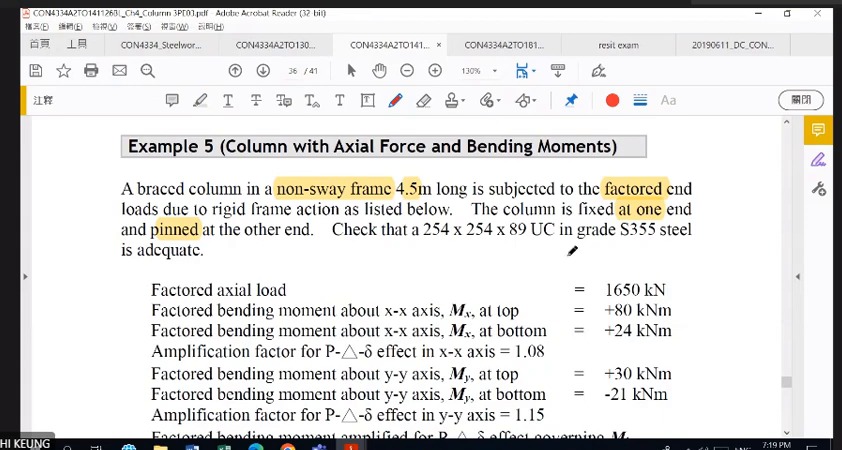
Example 5: given conditions for a non-sway-frame column
The column is in a non-sway frame, fixed at one end and pinned at the other, with axial force . End moments are +80/+24 kNm about and +30/−21 kNm about .
Specified amplification factors are 1.08 about and 1.15 about , giving governing demands and .
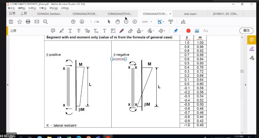
How to read this image: Read end-moment directions in the diagram before selecting . Do not rely solely on dividing the signed numbers in the question.
Example 5: section capacities and total utilisation
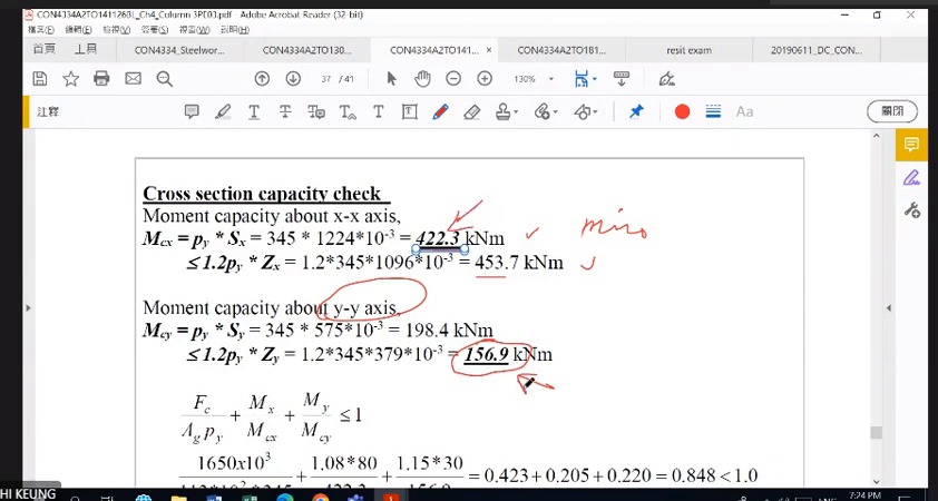
Thickness gives . For use ; for use .
. The axial ratio is about 0.423 and moment ratios about 0.205 and 0.220. Their sum is approximately 0.848<1, so the section passes.
Example 5: effective length, buckling curves and moment factors
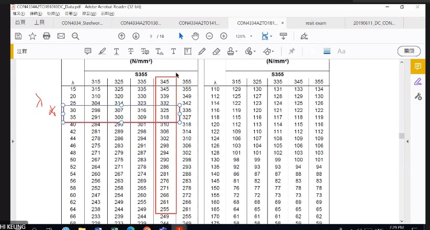
The end conditions give , and . The respective curves give about and ≈246 N/mm² about , so the weak axis governs.
The course moment-diagram ratios are with , and with .
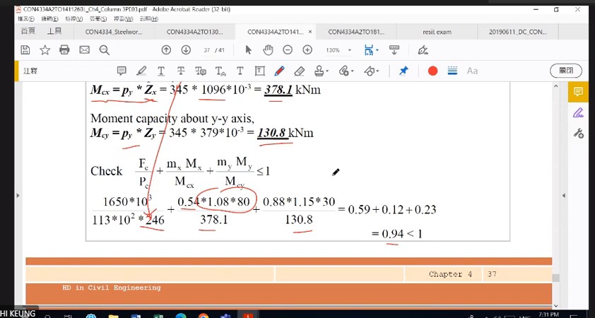
How to read this image: Read axial, and terms in sequence, checking , and elastic capacities 378.1/130.8.
Example 5: LTB resistance and member checks
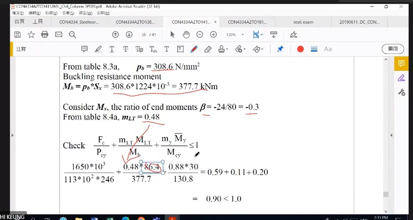
With , , , and , the screen obtains . The table gives and .
Member moment terms use elastic capacities and . With and , the first total is about 0.95. The LTB expression uses and totals about 0.94. Both are below 1.
Example 5: biaxial checks for a non-sway-frame column (Biaxial Column)
A 4.5 m column, 254×254×89 UC, is fixed at one end and pinned at the other. It carries 1650 kN of compression plus end moments about both axes. Decide whether the section is strong enough and whether the whole column buckles.
Solution Route: Amplify demand→classification/section capacities→section interaction→effective length /pc→moment factors→member interaction and LTB.
Q2: same section, new loading and effective length (Updated Column Inputs)
What this unit is for: The same section now has a new compression, new moments and a new effective length; this unit redoes the cross-section and whole-column checks, and the column only just passes.
Picture it this way: Start a fresh page with the new data and amplify the moments. The cross-section check uses ; the whole-column check switches to the smaller . With no information on how the moments vary, every m is taken as 1, which treats the moment as equally large all along the column, the worst case.
Prerequisites: Combined axial force and bending (Interaction Checks) · Instability can precede material crushing (Buckling)
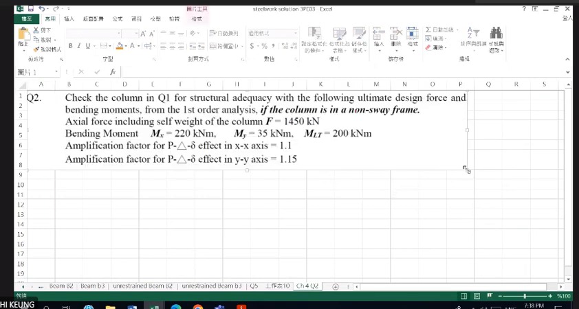
Q2 returns to 305×305×118 UC but changes axial force , moments and effective length : , , and . List the new data rather than copying Example 5 because the designation seems familiar.
Section utilisation is 0.8035. For the member, -axis gives and . No end-moment distribution is supplied, so is taken conservatively.
The member expressions give 0.988 and 0.992, both below 1. The column passes with little margin. The second uses LTB resistance , from and .
Complete worked examples in this unit: Column Q2: section and member checks for 305×305×118 UC (Column Q2)
Q2: add biaxial bending to the same section
Use 305×305×118 UC with , design axial force , , and governing .
Amplification factors 1.1 and 1.15 give demands 242 and 40.25 kNm. Treat LTB demand separately using the specified governing moment.
Q2: continue to buckling after the section check
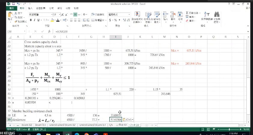
and . Section bending resistances are approximately 675.5 kNm about and 243.9 kNm about .
Using amplified moments gives section utilisation about 0.280+0.358+0.165=0.804<1. Next, and give for member checks.
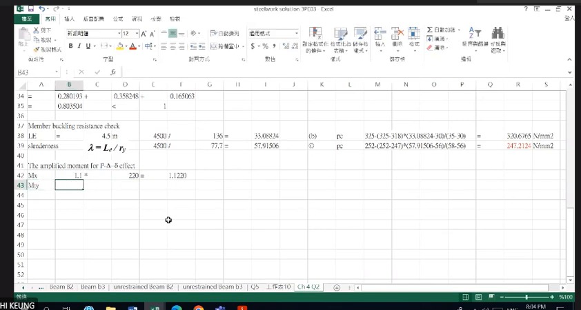
How to read this image: Curve b about gives ; curve c about gives 247.2 N/mm². Use the smaller.
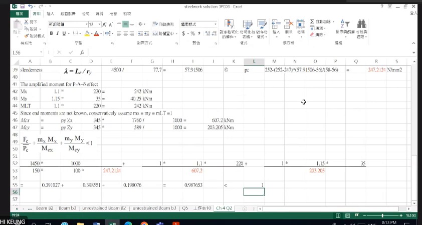
How to read this image: Use elastic denominators: and .
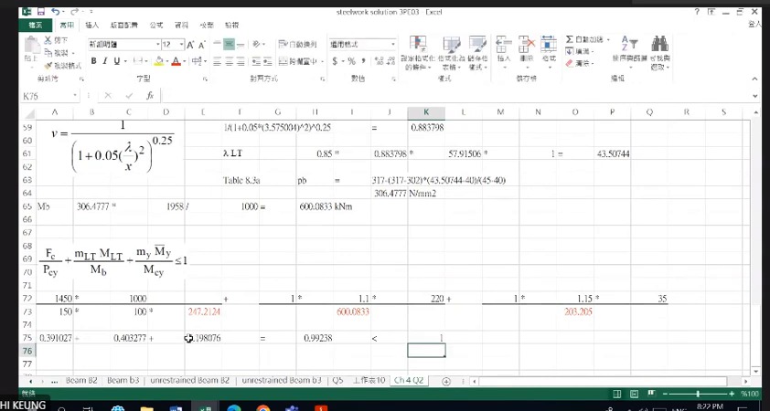
How to read this image: . Read , giving .
Column Q2: section and member checks for 305×305×118 UC (Column Q2)
A 305×305×118 UC column with an effective length of 4.5 m carries 1450 kN of compression and moments of 220 and 35 kNm about its two axes, before amplification. Complete the section check and both member checks to decide whether the column is adequate.
Solution Route: Amplify demand→section utilisation→two-axis →→first member expression→LTB resistance →second member expression.
Q3: a heavier section, all three checks (Heavier Section)
What this unit is for: A heavier section is used and the end moments change; this unit gets and m from the signs of the end moments, then completes the three checks.
Picture it this way: Write one line for each direction: the two end moments, the smaller divided by the larger to give , and m from the table. The factor m multiplies the demand only, while capacities such as and stay underneath. Each formula adds three ratios and compares the total with 1.
Prerequisites: Will the plate buckle before its material strength is fully mobilised? (Section Classification) · Combined axial force and bending (Interaction Checks) · Instability can precede material crushing (Buckling)
Q3 uses a heavier 305×305×198 UC and new loading: ; end moments +350/+150 kNm amplified by 1.1; end moments +90/−70 kNm amplified by 1.15; . Restate the conditions for every new problem, then follow the same procedure.
End-moment signs determine . Same-sign end moments give double curvature, , and . Opposite-sign moments give single curvature, and .
The section check is 0.853; member checks are 0.951 and 0.914. All are below 1, so the column passes. For , and . LTB uses , and .
Complete worked examples in this unit: Column Q3: biaxial bending of 305×305×198 UC (Column Q3)
Q3: complete procedure for a heavier UC section
The section changes to a heavier 305×305×198 UC with different end moments about both axes. Recalculate and ; do not retain Example 5 factors.
The sequence remains classification and →two-axis section capacities→→curves and →moment factors→two member interaction expressions.
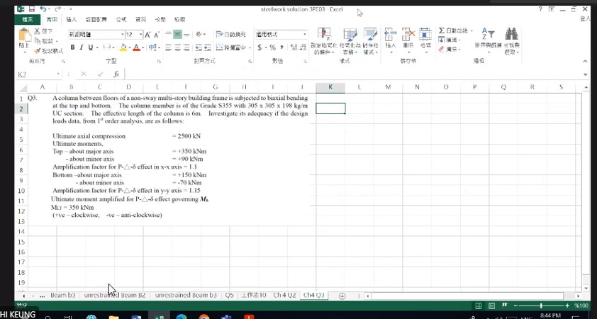
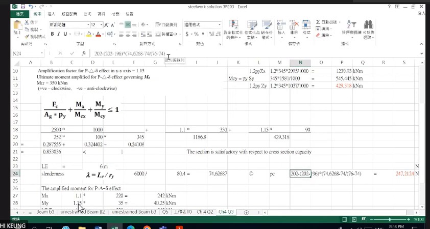
How to read this image: 2500/8694=0.288; 1.1×350/1186.8=0.324; 1.15×90/429.3=0.241.
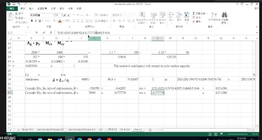
How to read this image: gives . gives ; gives .
Q3: put moment factors on the correct demand terms
and multiply moment demands. , or remain in their corresponding denominators. Every term must be dimensionless.
The worksheet shows and . These reflect different moment diagrams; do not set both to 1 merely because this is another column question.
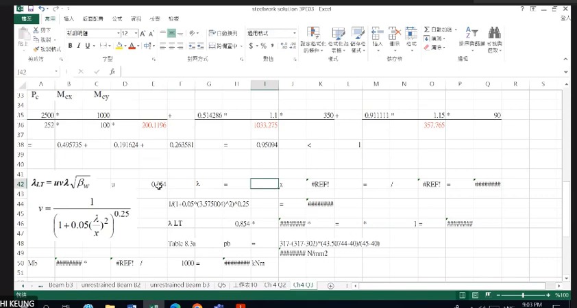
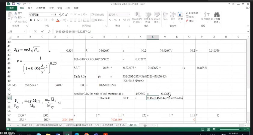
How to read this image: ^0.25≈0.722; .
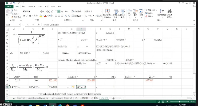
How to read this image: Multiply by , then divide by .
Column Q3: biaxial bending of 305×305×198 UC (Column Q3)
A 305×305×198 UC column with an effective length of 6 m carries 2500 kN of compression. End moments are 350 and 150 kNm about the axis, and 90 and −70 kNm about the axis. Complete the section check and both member checks.
Solution Route: Amplify demand→section resistance/utilisation→→ and m factors→first member expression→LTB→second member expression.
Q5: derive biaxial moments from eccentric reactions (Eccentric Column Reactions)
What this unit is for: Several beams rest on the column from different sides, each off the column centre; this unit adds them into the column compression and finds the moments about the two axes.
Picture it this way: A round table stands on one central leg with a weight on each side. All the weight goes down the leg, but only the difference between the two sides tries to tip the table. The moments from beam reactions on opposite sides of a column are likewise subtracted first, and only what remains bends the column.
Prerequisites: How loads travel from the slab to the ground (Load Path) · Why the position of a force matters (Moment and Eccentricity) · Combined axial force and bending (Interaction Checks)
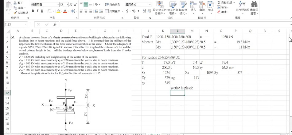
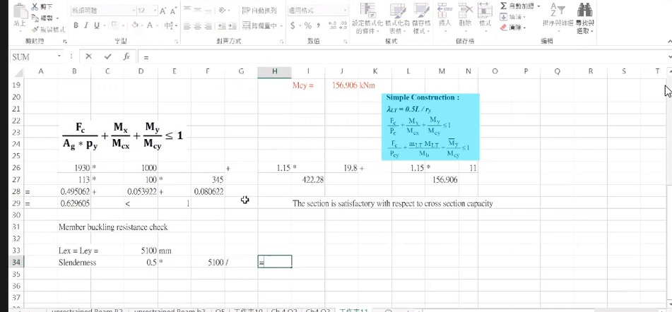
Add the five downward loads to obtain 1930 kN, then take moments about each axis. Subtract opposing rotations; do not make every force-times-distance term positive.
The upper and lower column segments have equal stiffness here, so divide net joint moment by 2. This differs from the previous 6 m/3 m distribution. Two segments do not always imply equal sharing.
After amplification by 1.15 about both axes, section utilisation is only 0.630. It appears generous, but 5100 mm length reduces . The next unit explains why member utilisation still exceeds 1.
Q5: how eccentric loads produce biaxial moments
Axial force is 1200+150+100+180+300=1930 kN.
The screen calculates and . Division by 2 follows this problem's upper/lower segment distribution assumption; it is not universal.
Q5: passing the section is only the first stage
For 254×254×89 UC, and ; section bending capacities are 422.3 and 156.9 kNm. Both moments are amplified by 1.15 to 22.77 and 12.65 kNm.
Section utilisation is about 0.495+0.054+0.081=0.630<1. However, and give , requiring reduced member resistance.
Q5 decision: a result slightly above 1 judged marginally OK (Interpreting a Marginal Result)
What this unit is for: The cross-section check has plenty to spare, yet both whole-column formulas come out slightly above 1; this unit explains how such a result should be written down.
Picture it this way: Both subjects must be passed, and a high mark in one cannot make up for just missing the other. A low ratio for the cross-section cannot make up for a whole-column ratio slightly above 1. The answer states the values of both formulas as they are, without rounding them down to 1.
Prerequisites: Combined axial force and bending (Interaction Checks) · Instability can precede material crushing (Buckling)
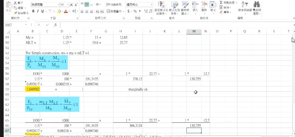
Using the same data, the two member checks give approximately 1.050 and 1.052, only about 5% above 1. The lecturer writes “marginally OK” beside the worksheet, judging it just acceptable. The section utilisation 0.630 cannot be used to offset the member checks.
In the exam, follow the lecturer: give the values of both expressions, then write “marginally OK”. Remark: under the strict ≤1 condition, 1.05 exceeds the limit, and the lecturer also says it is, in principle, not OK.
State which expression, its value and the limit exceeded. Any redesign requires a revised section or restraint and recalculation, not merely a changed conclusion.
Complete worked examples in this unit: Q5: utilisation slightly above 1, judged marginally OK by the lecturer (Marginal Utilization)
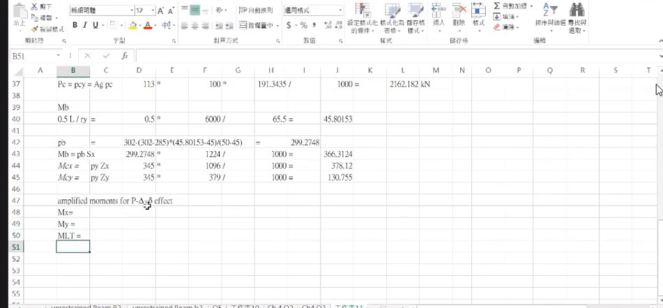
How to read this image: Confirm and the corresponding capacities before reading the next interaction screen. Do not mix in data from other 305-series sections.
Q5: slightly above 1, judged marginally OK by the lecturer
The course obtains and . Member elastic bending capacities are about 378.1 and 130.8 kNm. The simple-construction method uses moment factors of 1.
The first expression is approximately 1930/2162+22.77/378.1+12.65/130.8=1.050>1. The LTB expression uses and also totals about 1.05>1.
Both expressions exceed 1 by only about 5%. The lecturer writes “marginally OK” beside the worksheet, meaning just acceptable; in the answer, give the values of both expressions.
Q5: utilisation slightly above 1, judged marginally OK by the lecturer (Marginal Utilization)
A 254×254×89 UC column carries 1200 kN at its centre plus four downward forces that act away from the centre and so bend the column. Find the total compression and the moments about both axes, then check the section and the whole column.
Solution Route: Combine loads→eccentric moments→specified distribution→amplification→section check→two member checks→the lecturer's judgement.
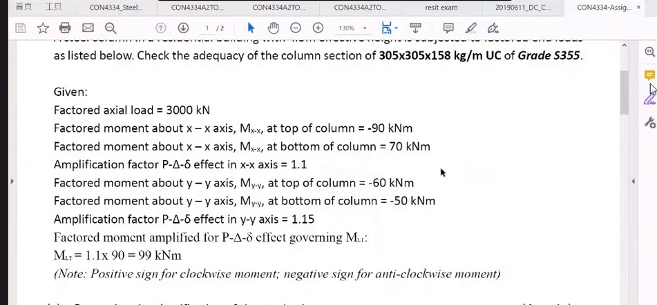
Final exercise: the 3000 kN column (End-of-lecture Question)
What this unit is for: A column question gives end moments with signs about both axes; this unit first turns them into amplified moments and values, ready for the interaction check.
Picture it this way: Copy the two end moments for each direction on its own line, signs included. On each line the larger one times the amplification factor is the demand, and the smaller divided by the larger gives . These numbers alone settle nothing, because the capacities have not been worked out yet.
Prerequisites: Combined axial force and bending (Interaction Checks) · Why the position of a force matters (Moment and Eccentricity)
The lecturer ends with a past-paper question: 305×305×158 UC, S355, ; end moments −90/+70 kNm amplified by 1.1; end moments −60/−50 kNm amplified by 1.15; .
List signed end moments by axis, then obtain amplified governing values and . Retain signs because they determine : opposite-sign moments give single curvature and ; same-sign moments give double curvature and .
Only the -to-m lookup is shown here. The 14 November revision uses the same 3000 kN, 99 kNm and 69 kNm actions for interaction checks; see its assignment-beams-and-columns unit.
Final exercise: organise signed end moments first
Given end moments are −90/+70 kNm about and −60/−50 kNm about . Amplification factors are 1.1 and 1.15, with governing .
First obtain maximum absolute demands and . Then use the moment diagrams to establish and factors, complete both-axis lookups and interaction checks.