Worked Example

Column Q2: section and member checks for 305×305×118 UC (Column Q2)

Task: Complete the section check and both member checks to determine whether the column passes.

Original question · Lecture notes Chapter 4, p. 40 (Tutorial 4 Q1–Q2)
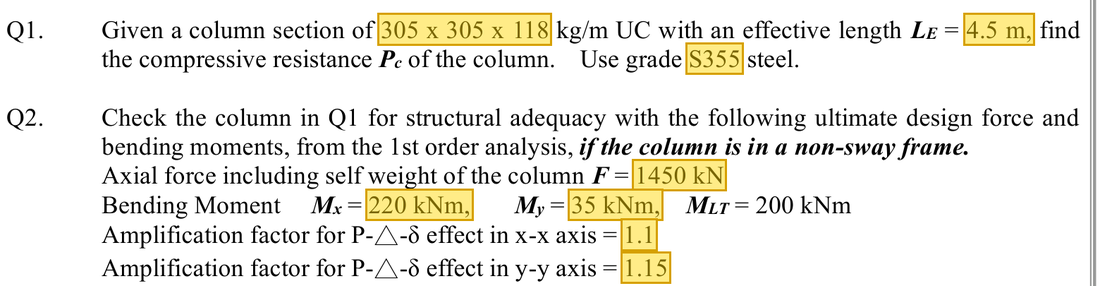
Original question with the given values boxed
Yellow boxes: values the question gives, the same values marked yellow in the Given table below.

The question in short: A 305×305×118 UC column with an effective length of 4.5 m carries 1450 kN of compression and moments of 220 and 35 kNm about its two axes, before amplification. Complete the section check and both member checks to decide whether the column is adequate.

What differs from the previous example of this type: The route is the same as the previous example, but the section is larger and the end-moment pattern is not given. So mxm_x, mym_y and mLTm_{LT} are all taken as 1, meaning the moments are not reduced at all.

GivenValue and Unit
Section305×305×118 UC, S355; Ag=150 cm2\htmlClass{read}{A_g=150\ \mathrm{cm^{2}}}; Sx=1958\htmlClass{read}{S_x=1958}, Sy=895\htmlClass{read}{S_y=895}, Zx=1760\htmlClass{read}{Z_x=1760}, Zy=589 cm3\htmlClass{read}{Z_y=589\ \mathrm{cm^{3}}}; rx=136\htmlClass{read}{r_x=136}, ry=77.7 mm\htmlClass{read}{r_y=77.7\ \mathrm{mm}}; py=345 N/mm2\htmlClass{read}{p_y=345\ \mathrm{N/mm^{2}}}
DemandFc=1450 kN\htmlClass{given}{F_c=1450\ \mathrm{kN}}; Mx=220\htmlClass{given}{M_x=220} and My=35 kNm\htmlClass{given}{M_y=35\ \mathrm{kNm}}, amplified by 1.1 and 1.15; MLTM_{LT} follows the lecturer's worksheet at 1.1×220=242 kNm
Member dataLe=4.5 m\htmlClass{given}{L_e=4.5\ \mathrm{m}}; u=0.85\htmlClass{read}{u=0.85}; x=16.2\htmlClass{read}{x=16.2}; unknown end-moment distribution, so mx=my=mLT=1m_x=m_y=m_{LT}=1

Yellow: values given in the question. The same values are marked where they are substituted in the steps below.
Orange box: values read directly from the Data File, the same values boxed orange in the lookup screenshots. A value interpolated between two table rows is a calculation, so it has no box.

Data file lookup · Data Page 11 · Universal Columns — Properties
305×305×118 UC: rx = 13.6 cm, ry = 7.77 cm, Zx = 1760, Zy = 589, Sx = 1958, Sy = 895 cm³, u = 0.850, x = 16.2, A = 150 cm².
305×305×118 UC: rx=13.6 cmr_x=13.6\ \mathrm{cm}, ry=7.77 cmr_y=7.77\ \mathrm{cm}, Zx=1760Z_x=1760, Zy=589Z_y=589, Sx=1958S_x=1958, Sy=895 cm3S_y=895\ \mathrm{cm^{3}}, u=0.850u=0.850, x=16.2x=16.2, A=150 cm2A=150\ \mathrm{cm^{2}}.Yellow: given parameter, row or columnOrange: value read from the table, boxed orange in the text too
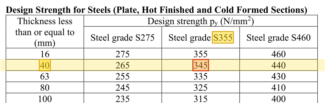
Data file lookup · Data Page 1 · Design strength pyp_y
Flange T = 18.7 mm thick: the T ≤ 40 mm row, S355 column gives py = 345 N/mm².
Flange T=18.7 mmT=18.7\ \mathrm{mm} thick: the T≤40 mmT\le40\ \mathrm{mm} row, S355 column gives py=345 N/mm2p_y=345\ \mathrm{N/mm^{2}}. How the grade and thickness choose this row →Yellow: given parameter, row or columnOrange: value read from the table, boxed orange in the text too

Solution Route: Amplify demand→section utilisation→two-axis λ/pc\lambda/p_c→PcP_c→first member expression→LTB resistance MbM_b→second member expression.

Load path · the stations the force passes through, in order

Axial force and moments about both axes act on the column together. Their three ratios must add up to no more than 1, checked once with the section capacities and once with each buckling capacity.

  1. Axial force and amplified moments
    Fc=1450 kNF_c=1450\ \mathrm{kN}; Mx=242M_x=242, My=40.25 kNmM_y=40.25\ \mathrm{kNm}
  2. Cross-section check
    Sum 0.8035Limit 1
  3. Member check 1 (buckling)
    Sum 0.988Limit 1
  4. Member check 2 (lateral-torsional buckling)
    Sum 0.992Limit 1
    closest to the limit
Red frame: the station closest to its limit. Each station links to the step that calculates it.
  1. Step 1 · Amplify demand

    Why this step: Once the compressed column deforms, the moments become somewhat larger than first calculated. Each moment is amplified first, and every later check uses the amplified values.

    The axes use different amplification factors.

    New symbols in this step
    • MxM_x, MyM_y, MLTM_{LT}: Two-axis and LTB governing moment demands; kNm
    • kxk_x, kyk_y, Mx1M_{x1}, My1M_{y1}: Amplification factors for the two axes; larger end moment before amplification, kNm
    Mx=kxMx1=1.1(220)=242,My=kyMy1=1.15(35)=40.25 kNmM_x=k_xM_{x1}={\htmlClass{given}{1.1}}({\htmlClass{given}{220}})=242,\qquad M_y=k_yM_{y1}={\htmlClass{given}{1.15}}({\htmlClass{given}{35}})=40.25\ \mathrm{kNm}
    Mx=kxMx1=1.1(220)=242My=kyMy1=1.15(35)=40.25 kNm\begin{aligned}M_x&=k_xM_{x1}={\htmlClass{given}{1.1}}({\htmlClass{given}{220}})=242\\M_y&=k_yM_{y1}={\htmlClass{given}{1.15}}({\htmlClass{given}{35}})=40.25\ \mathrm{kNm}\end{aligned}

    ▶ The lecturer on this part: 31 October 00:44:58

  2. Step 2 · Section check

    Why this step: This first confirms that the hardest-worked cross-section is not crushed. Column length plays no part here; if the section itself fails, there is no point going on to buckling.

    Area 150 cm² = 15000 mm²; each moment capacity McM_c is the smaller of pySp_yS and 1.2pyZ, then each demand is divided by its section capacity.

    New symbols in this step
    • FcF_c, PcP_c: Design axial force and buckling compression resistance; kN
    • AgA_g, pyp_y, pcp_c: Gross area mm²; yield and compression buckling strengths N/mm²
    • McxM_{cx}, McyM_{cy}, MbM_b: Corresponding bending resistances; kNm, with different section/member definitions
    Agpy=150(100)(345)/1000=5175 kNMcx=min⁡(345(1958), 1.2(345)(1760))/1000=675.5 kNmMcy=min⁡(345(895), 1.2(345)(589))/1000=243.8 kNmηs=FcAgpy+MxMcx+MyMcy=14505175+242675.5+40.25243.8≈0.8035<1\begin{aligned}A_gp_y&={\htmlClass{read}{150}}(100)({\htmlClass{read}{345}})/1000=5175\ \mathrm{kN}\\M_{cx}&=\min({\htmlClass{read}{345}}({\htmlClass{read}{1958}}),\ 1.2({\htmlClass{read}{345}})({\htmlClass{read}{1760}}))/1000=675.5\ \mathrm{kNm}\\M_{cy}&=\min({\htmlClass{read}{345}}({\htmlClass{read}{895}}),\ 1.2({\htmlClass{read}{345}})({\htmlClass{read}{589}}))/1000=243.8\ \mathrm{kNm}\\\eta_s&=\frac{F_c}{A_gp_y}+\frac{M_x}{M_{cx}}+\frac{M_y}{M_{cy}}\\&=\frac{{\htmlClass{given}{1450}}}{5175}+\frac{242}{675.5}+\frac{40.25}{243.8}\approx0.8035<1\end{aligned}
    Agpy=150(100)(345)/1000=5175 kNMcx=min⁡(345(1958), 1.2(345)(1760))/1000=675.5 kNmMcy=min⁡(345(895), 1.2(345)(589))/1000=243.8 kNmηs=FcAgpy+MxMcx+MyMcy=14505175+242675.5+40.25243.8≈0.8035<1\begin{aligned}A_gp_y&={\htmlClass{read}{150}}(100)({\htmlClass{read}{345}})/1000\\&=5175\ \mathrm{kN}\\M_{cx}&=\min({\htmlClass{read}{345}}({\htmlClass{read}{1958}}),\\&\quad \ 1.2({\htmlClass{read}{345}})({\htmlClass{read}{1760}}))/1000\\&=675.5\ \mathrm{kNm}\\M_{cy}&=\min({\htmlClass{read}{345}}({\htmlClass{read}{895}}),\\&\quad \ 1.2({\htmlClass{read}{345}})({\htmlClass{read}{589}}))/1000\\&=243.8\ \mathrm{kNm}\\\eta_s&=\frac{F_c}{A_gp_y}+\frac{M_x}{M_{cx}}+\frac{M_y}{M_{cy}}\\&=\frac{{\htmlClass{given}{1450}}}{5175}+\frac{242}{675.5}+\frac{40.25}{243.8}\\&\approx0.8035\\&<1\end{aligned}

    Where the numbers come from: 40.2540.25 from Step 1.

    Units: AgA_g is multiplied by 100 to change cm² into mm²; times pyp_y gives N, and dividing by 1000 gives kN. SS and ZZ are multiplied by 1000 to change cm³ into mm³; Nmm divided by 1000000 gives kNm, a net division by 1000.

    ▶ The lecturer on this part: 31 October 01:04:55

  3. Step 3 · Slenderness about both axes

    Why this step: The column can bow about the xx axis or the yy axis, so pcp_c is found for each. The smaller ryr_y gives the yy axis the larger slenderness and the lower pcp_c.

    Use curve b about xx and curve c about yy, interpolating each in the py=345p_y=345 column.

    New symbols in this step
    • LeL_e, rxr_x, ryr_y, λ\lambda: Effective length and radius of gyration mm; dimensionless slenderness
    λx=LE/rx=4500/136=33.1pcx=325+33.1−3035−30(318−325)≈320.7 N/mm2λy=LE/ry=4500/77.7=57.9pcy=252+57.9−5658−56(247−252)≈247.2 N/mm2\begin{aligned}\lambda_x&=L_E/r_x={\htmlClass{given}{4500}}/{\htmlClass{read}{136}}=33.1\\p_{cx}&={\htmlClass{read}{325}}+\frac{33.1-{\htmlClass{given}{30}}}{{\htmlClass{given}{35}}-{\htmlClass{given}{30}}}({\htmlClass{read}{318}}-{\htmlClass{read}{325}})\approx320.7\ \mathrm{N/mm^2}\\\lambda_y&=L_E/r_y={\htmlClass{given}{4500}}/{\htmlClass{read}{77.7}}=57.9\\p_{cy}&={\htmlClass{read}{252}}+\frac{57.9-{\htmlClass{given}{56}}}{{\htmlClass{given}{58}}-{\htmlClass{given}{56}}}({\htmlClass{read}{247}}-{\htmlClass{read}{252}})\approx247.2\ \mathrm{N/mm^2}\end{aligned}
    λx=LE/rx=4500/136=33.1pcx=325+33.1−3035−30(318−325)≈320.7 N/mm2λy=LE/ry=4500/77.7=57.9pcy=252+57.9−5658−56(247−252)≈247.2 N/mm2\begin{aligned}\lambda_x&=L_E/r_x={\htmlClass{given}{4500}}/{\htmlClass{read}{136}}=33.1\\p_{cx}&={\htmlClass{read}{325}}+\frac{33.1-{\htmlClass{given}{30}}}{{\htmlClass{given}{35}}-{\htmlClass{given}{30}}}({\htmlClass{read}{318}}-{\htmlClass{read}{325}})\\&\approx320.7\ \mathrm{N/mm^2}\\\lambda_y&=L_E/r_y={\htmlClass{given}{4500}}/{\htmlClass{read}{77.7}}=57.9\\p_{cy}&={\htmlClass{read}{252}}+\frac{57.9-{\htmlClass{given}{56}}}{{\htmlClass{given}{58}}-{\htmlClass{given}{56}}}({\htmlClass{read}{247}}-{\htmlClass{read}{252}})\\&\approx247.2\ \mathrm{N/mm^2}\end{aligned}

    Units: The 4.5 m effective length is multiplied by 1000 to give 4500 mm and divided by rxr_x and ryr_y in mm. Millimetres divided by millimetres leave slenderness with no unit.

    Data file lookup · Data Page 7 · Table 8.7 Buckling curves
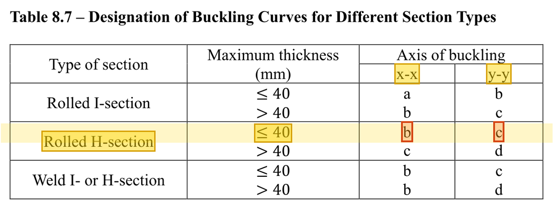
    Rolled H-section with thickness ≤ 40 mm: use curve b about the x-x axis and curve c about the y-y axis.
    Rolled H-section with thickness ≤ 40 mm: use curve b about the x-xx\text{-}x axis and curve c about the y-yy\text{-}y axis.Yellow: given parameter, row or columnOrange: value read from the table, boxed orange in the text too
    Data file lookup · Data Page 8 · Table 8.8(b)
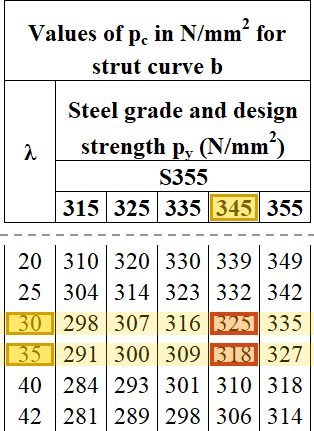
    Table 8.8(b) (x axis, curve b), py = 345 column: λ = 30 → 325 and λ = 35 → 318 N/mm²; interpolating at λx = 33.1 gives pc ≈ 320.7 N/mm².
    Table 8.8(b) (xx axis, curve b), py=345p_y=345 column: λ=30\lambda=30 → 325 and λ=35\lambda=35 → 318 N/mm²; interpolating at λx=33.1\lambda_{x}=33.1 gives pc≈320.7 N/mm2p_c\approx320.7\ \mathrm{N/mm^{2}}.Yellow: given parameter, row or columnOrange: value read from the table, boxed orange in the text too
    Data file lookup · Data Page 8 · Table 8.8(c)
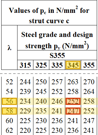
    Table 8.8(c) (y axis, curve c), py = 345 column: λ = 56 → 252 and λ = 58 → 247 N/mm²; interpolating at λy = 57.9 gives pc ≈ 247.2 N/mm².
    Table 8.8(c) (yy axis, curve c), py=345p_y=345 column: λ=56\lambda=56 → 252 and λ=58\lambda=58 → 247 N/mm²; interpolating at λy=57.9\lambda_{y}=57.9 gives pc≈247.2 N/mm2p_c\approx247.2\ \mathrm{N/mm^{2}}.Yellow: given parameter, row or columnOrange: value read from the table, boxed orange in the text too

    ▶ The lecturer on this part: 31 October 01:09:59

  4. Step 4 · Buckling resistance

    Why this step: PcP_c is the force the whole column can carry before it bows about the weak axis. It is smaller than the crushing value AgpyA_gp_y; the difference comes from the length of the column.

    Take the smaller pcp_c.

    Pc=Agpcy=150(100)(247.2)/1000≈3708 kNP_c=A_gp_{cy}={\htmlClass{read}{150}}(100)(247.2)/1000\approx3708\ \mathrm{kN}
    Pc=Agpcy=150(100)(247.2)/1000≈3708 kN\begin{aligned}P_c&=A_gp_{cy}\\&={\htmlClass{read}{150}}(100)(247.2)/1000\\&\approx3708\ \mathrm{kN}\end{aligned}

    Where the numbers come from: 247.2247.2 from Step 3.

    Units: AgA_g of 150 cm² is multiplied by 100 to change it into mm². pcp_c in N/mm² times mm² gives N, and dividing by 1000 gives kN.

  5. Step 5 · Elastic capacities

    Why this step: The member checks do not let the section go plastic. They stop when the outermost steel just reaches pyp_y, so the moment capacities are a little smaller than in the section check.

    Member-expression denominators use pyZp_yZ.

    Mcx=pyZx=345(1760)/1000=607.2 kNmMcy=pyZy=345(589)/1000=203.2 kNm\begin{aligned}M_{cx}&=p_yZ_x={\htmlClass{read}{345}}({\htmlClass{read}{1760}})/1000=607.2\ \mathrm{kNm}\\M_{cy}&=p_yZ_y={\htmlClass{read}{345}}({\htmlClass{read}{589}})/1000=203.2\ \mathrm{kNm}\end{aligned}
    Mcx=pyZx=345(1760)/1000=607.2 kNmMcy=pyZy=345(589)/1000=203.2 kNm\begin{aligned}M_{cx}&=p_yZ_x\\&={\htmlClass{read}{345}}({\htmlClass{read}{1760}})/1000\\&=607.2\ \mathrm{kNm}\\M_{cy}&=p_yZ_y\\&={\htmlClass{read}{345}}({\htmlClass{read}{589}})/1000\\&=203.2\ \mathrm{kNm}\end{aligned}

    Units: ZxZ_x and ZyZ_y are multiplied by 1000 to change cm³ into mm³. pyp_y times mm³ gives Nmm, and dividing by 1000000 gives kNm. Together this is a division by 1000.

    ▶ The lecturer on this part: 31 October 01:18:15

  6. Step 6 · First member expression

    Why this step: Taking m as 1 assumes the largest moment acts along the whole column, which is the most cautious choice. A total close to 1 means the buckling capacity of the column is almost fully used.

    No end-moment distribution is supplied, so take mx=my=1m_x=m_y=1.

    New symbols in this step
    • mxm_x, mym_y, mLTm_{LT}: Equivalent moment-distribution factors; dimensionless
    FcPc+mxMxpyZx+myMypyZy=14503708+242607.2+40.25203.2=0.391+0.399+0.198≈0.988<1\begin{aligned}&\frac{F_c}{P_c}+\frac{m_xM_x}{p_yZ_x}+\frac{m_yM_y}{p_yZ_y}\\&=\frac{{\htmlClass{given}{1450}}}{3708}+\frac{242}{607.2}+\frac{40.25}{203.2}\\&=0.391+0.399+0.198\approx0.988<1\end{aligned}
    FcPc+mxMxpyZx+myMypyZy=14503708+242607.2+40.25203.2=0.391+0.399+0.198≈0.988<1\begin{aligned}&\frac{F_c}{P_c}+\frac{m_xM_x}{p_yZ_x}+\frac{m_yM_y}{p_yZ_y}\\&=\frac{{\htmlClass{given}{1450}}}{3708}+\frac{242}{607.2}+\frac{40.25}{203.2}\\&=0.391+0.399+0.198\\&\approx0.988\\&<1\end{aligned}

    Where the numbers come from: 37083708 from Step 4; 607.2607.2 from Step 5; 40.2540.25 from Step 1; 203.2203.2 from Step 5.

  7. Step 7 · LTB resistance

    Why this step: Under the moment about the xx axis the column behaves like a beam, and its compression flange can move sideways. The weak-axis slenderness is used because that sideways movement is bending about the weak axis.

    Calculate λLT=uvλβw\lambda_{LT}=uv\lambda\sqrt{\beta_{w}}, then consult Table 8.3a.

    v=1(1+0.05(λ/x)2)0.25=1(1+0.05(57.9/16.2)2)0.25=0.884λLT=uvλ=0.85(0.884)(57.9)≈43.5\begin{aligned}v&=\frac{1}{(1+0.05(\lambda/x)^2)^{0.25}}\\&=\frac{1}{(1+0.05(57.9/{\htmlClass{read}{16.2}})^2)^{0.25}}=0.884\\\lambda_{LT}&=uv\lambda={\htmlClass{read}{0.85}}(0.884)(57.9)\approx43.5\end{aligned}
    v=1(1+0.05(λ/x)2)0.25=1(1+0.05(57.9/16.2)2)0.25=0.884λLT=uvλ=0.85(0.884)(57.9)≈43.5\begin{aligned}v&=\frac{1}{(1+0.05(\lambda/x)^2)^{0.25}}\\&=\frac{1}{(1+0.05(57.9/{\htmlClass{read}{16.2}})^2)^{0.25}}=0.884\\\lambda_{LT}&=uv\lambda\\&={\htmlClass{read}{0.85}}(0.884)(57.9)\\&\approx43.5\end{aligned}

    Where the numbers come from: 57.957.9 from Step 3.

    ▶ The lecturer on this part: 31 October 01:27:52

  8. Step 8 · Find pbp_b and MbM_b

    Why this step: MbM_b is the moment the column, treated as a beam, can carry before it moves sideways and twists. It is slightly below pyZxp_yZ_x, so the second check comes out a little stricter than the first.

    For py=345p_y=345, λLT=40\lambda_{LT}=40 gives 317 and 45 gives 302. Interpolate between them.

    New symbols in this step
    • λ1\lambda_1, λ2\lambda_2, p1p_1, p2p_2: Slenderness and table values of the two rows used for interpolation
    pb=p1+λLT−λ1λ2−λ1(p2−p1)=317+43.5−4045−40(302−317)≈306.5 N/mm2Mb=pbSx=306.5(1958)/1000≈600.1 kNm\begin{aligned}p_b&=p_1+\frac{\lambda_{LT}-\lambda_1}{\lambda_2-\lambda_1}(p_2-p_1)\\&={\htmlClass{read}{317}}+\frac{43.5-{\htmlClass{given}{40}}}{{\htmlClass{given}{45}}-{\htmlClass{given}{40}}}({\htmlClass{read}{302}}-{\htmlClass{read}{317}})\approx306.5\ \mathrm{N/mm^2}\\M_b&=p_bS_x=306.5({\htmlClass{read}{1958}})/1000\approx600.1\ \mathrm{kNm}\end{aligned}
    pb=p1+λLT−λ1λ2−λ1(p2−p1)=317+43.5−4045−40(302−317)≈306.5 N/mm2Mb=pbSx=306.5(1958)/1000≈600.1 kNm\begin{aligned}p_b&=p_1+\frac{\lambda_{LT}-\lambda_1}{\lambda_2-\lambda_1}(p_2-p_1)\\&={\htmlClass{read}{317}}+\frac{43.5-{\htmlClass{given}{40}}}{{\htmlClass{given}{45}}-{\htmlClass{given}{40}}}({\htmlClass{read}{302}}-{\htmlClass{read}{317}})\\&\approx306.5\ \mathrm{N/mm^2}\\M_b&=p_bS_x\\&=306.5({\htmlClass{read}{1958}})/1000\\&\approx600.1\ \mathrm{kNm}\end{aligned}

    Where the numbers come from: 43.543.5 from Step 7.

    Units: SxS_x is multiplied by 1000 to change cm³ into mm³. pbp_b in N/mm² times mm³ gives Nmm, and dividing by 1000000 gives kNm, so the formula divides by 1000.

    Data file lookup · Data Page 5 · Table 8.3a
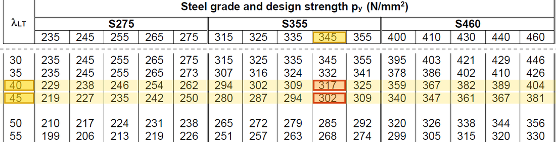
    Table 8.3a, py = 345 column: λLT = 40 → 317 and λLT = 45 → 302 N/mm²; interpolating at λLT = 43.5 gives pb ≈ 306.5 N/mm².
    Table 8.3a, py=345p_y=345 column: λLT=40\lambda_{LT}=40 → 317 and λLT=45\lambda_{LT}=45 → 302 N/mm²; interpolating at λLT=43.5\lambda_{LT}=43.5 gives pb≈306.5 N/mm2p_b\approx306.5\ \mathrm{N/mm^{2}}.Yellow: given parameter, row or columnOrange: value read from the table, boxed orange in the text too
  9. Step 9 · Second member expression

    Why this step: This check guards against the column bowing under compression while the strong-axis moment makes it move sideways and twist. Both member checks must be below 1 for the column to be stable.

    mLT=1m_{LT}=1, MLT=242 kNmM_{LT}=242\ \mathrm{kNm}.

    FcPc+mLTMLTMb+myMypyZy=14503708+242600.1+40.25203.2=0.391+0.403+0.198≈0.992<1\begin{aligned}&\frac{F_c}{P_c}+\frac{m_{LT}M_{LT}}{M_b}+\frac{m_yM_y}{p_yZ_y}\\&=\frac{{\htmlClass{given}{1450}}}{3708}+\frac{242}{600.1}+\frac{40.25}{203.2}\\&=0.391+0.403+0.198\approx0.992<1\end{aligned}
    FcPc+mLTMLTMb+myMypyZy=14503708+242600.1+40.25203.2=0.391+0.403+0.198≈0.992<1\begin{aligned}&\frac{F_c}{P_c}+\frac{m_{LT}M_{LT}}{M_b}+\frac{m_yM_y}{p_yZ_y}\\&=\frac{{\htmlClass{given}{1450}}}{3708}+\frac{242}{600.1}+\frac{40.25}{203.2}\\&=0.391+0.403+0.198\\&\approx0.992\\&<1\end{aligned}

    Where the numbers come from: 37083708 from Step 4; 600.1600.1 from Step 8; 40.2540.25 from Step 1; 203.2203.2 from Step 5.

    Load path · How the ratios add up
    Limit 1Cross-section0.280.3580.165≈ 0.8035Member 1 (buckling)0.3910.3990.198≈ 0.988Member 2 (LTB)0.3910.4030.198≈ 0.992Axial termx-axis moment termy-axis moment term
    Each bar is one check: blue is the share used by the axial force, green and yellow the shares used by the moments about the two axes. Together they must not pass the red dashed line.
Conclusion

Section utilisation 0.8035 and member utilisations 0.988/0.992 are all below 1. The column passes with little margin. The question gives MLT=200 kNmM_{LT}=200\ \mathrm{kNm}; using 1.1×200=220 kNm gives about 0.956 for the second expression, with the same conclusion.

All the symbols of this example

SymbolsMeaning and Units
FcF_c, PcP_cDesign axial force and buckling compression resistance; kN
AgA_g, pyp_y, pcp_cGross area mm²; yield and compression buckling strengths N/mm²
LeL_e, rxr_x, ryr_y, λ\lambdaEffective length and radius of gyration mm; dimensionless slenderness
MxM_x, MyM_y, MLTM_{LT}Two-axis and LTB governing moment demands; kNm
SxS_x, SyS_y, ZxZ_x, ZyZ_yTwo-axis plastic/elastic moduli; convert the tabulated cm³
McxM_{cx}, McyM_{cy}, MbM_bCorresponding bending resistances; kNm, with different section/member definitions
mxm_x, mym_y, mLTm_{LT}Equivalent moment-distribution factors; dimensionless
ηs\eta_s, η1\eta_1, η2\eta_2Total utilisations for the section and two member expressions; dimensionless
kxk_x, kyk_y, Mx1M_{x1}, My1M_{y1}Amplification factors for the two axes; larger end moment before amplification, kNm
λ1\lambda_1, λ2\lambda_2, p1p_1, p2p_2Slenderness and table values of the two rows used for interpolation

Video positions: 31 October 00:45:00 · 31 October 01:05:00 · 31 October 01:10:00 · 31 October 01:20:00 · 31 October 01:28:00

↑ Top