Final revision: selecting formulas for welds, bolts, beams and columns
The final lecture integrates formula sheets, tutorials and past papers. It changes questions quickly. Beginners should complete the earlier worked examples, then use this lecture for revision by problem type. Each dataset is listed separately; adjacent screens are not necessarily one problem.
Abbreviations: DL—Dead Load; LL—Live Load; ULS—Ultimate Limit State; SLS—Serviceability Limit State; UDL—Uniformly Distributed Load; LTB—Lateral-torsional Buckling; UB—Universal Beam; UC—Universal Column.
Key Points
- Identify each formula's model: UDL or point load, simply supported or overhanging, low or high shear.
- Classification limits use . Higher gives smaller and stricter limits.
- Connections: lap welds share equally; angle welds follow centroid position; plate bearing takes the minimum of four bounds.
- Class 1 describes local buckling behaviour, not immunity to LTB.
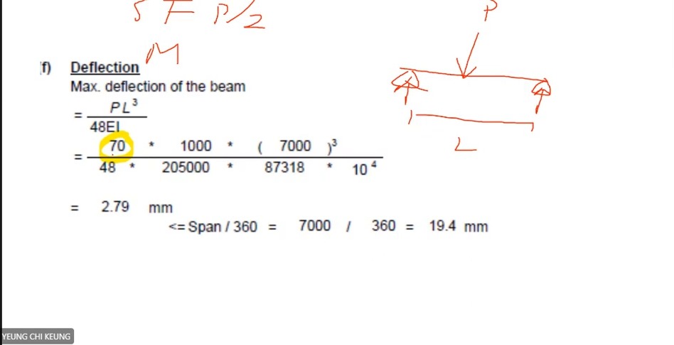
- Convert deflection inputs to N and mm, then compare with limits such as .
Key Formulas
Exam Question Types
- The four M27 plate-bearing bounds. → M27 plate bearing: calculate all four bounds (Four Bearing Limits)
- Floor-beam coexisting shear and deflection. → 6 m revision beam: coexisting shear and deflection (Coexistent Shear)
- Column interaction revision. → Column interaction revision: where each ratio comes from (Column Interaction Review)
Design flows for these question types
- The lecturer switches between old questions; each problem's data are listed separately here.
- Approximately 01:25–01:50 is a break. During it the lecturer shows another past-paper column question, BQ2 with 2400 kN, without solving it.
- Minor unit or layout errors in the lecturer's tables are corrected here by dimensional reasoning.
Read conditions together with formulas (Formula Conditions)
What this unit is for: Every formula applies only to a particular support, load or section condition; this unit revises those conditions and how to read the section classification table.
Picture it this way: Take the same thin plate. The stronger the steel, the higher the stress the plate is expected to reach, and the more likely it wrinkles before getting there. So for higher-strength steel the width-to-thickness limits become stricter, not looser.
Prerequisites: Will the plate buckle before its material strength is fully mobilised? (Section Classification) · Read an I-section and its section table (Section Properties) · Excessive bending deformation versus insufficient resistance (Deflection)
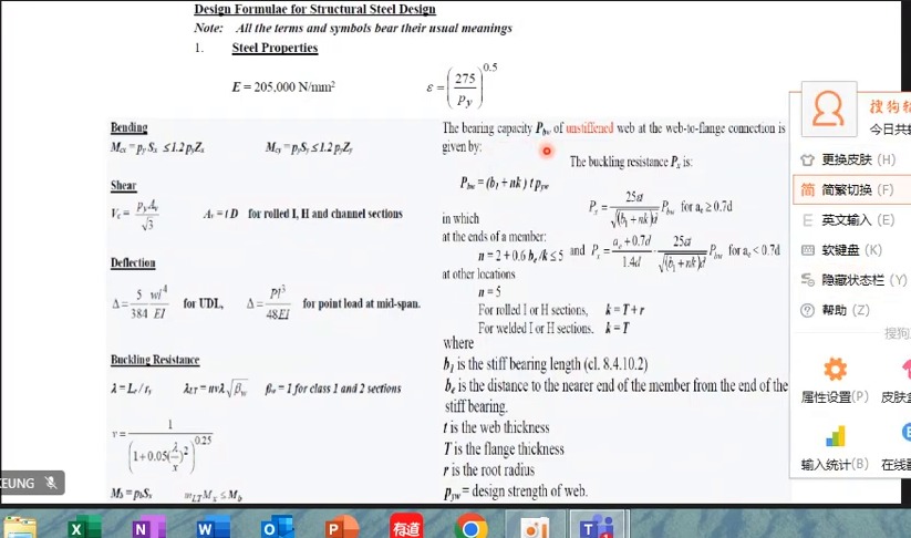
As the lecturer reviews the formula sheet, identify each model: simply supported full-span UDL, central point load, low-shear Class 1/2 or local web compression. A formula name is not its complete applicability condition; read supports and loading diagrams too.
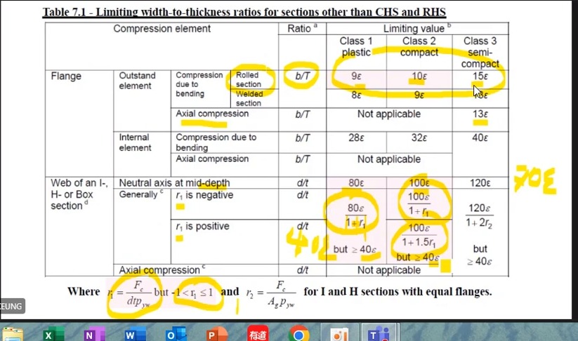
Classification rows distinguish rolled/welded manufacture, compressed plate type and stress distribution. Flange limits 9ε, 10ε and 15ε apply to specific rows. Web bending and axial compression differ; 80ε is not universal.
The assignment table shows that changing grade while keeping dimensions can reduce and worsen classification. Higher strength does not guarantee greater plastic development; compare geometry and strength together.
Formula sheet: confirm symbols and units first
The course uses and . is plastic section modulus; is elastic section modulus.
Match deflection expressions to supports and loading: full-span UDL and central point loads use different formulas. Local web bearing /buckling also requires bearing length, web thickness and flange–web junction dimensions.
Classification: do not memorise only one limit set
For the displayed rolled outstand compression flange in bending, Class 1/2/3 limits are 9ε, 10ε and 15ε. The corresponding welded-section row differs.
Web classification also depends on neutral-axis position and axial compression proportion. The screen bounds between −1 and 1. Do not use without identifying the stress state.
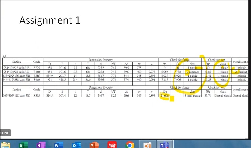
How to read this image: For each row, read and , then flange and web classes. Use the less favourable class overall.
Weld and bolt revision: identify the current problem (Connection Revision)
What this unit is for: The weld and bolt questions use similar formulas under different conditions; this unit revises them by first pinning down the load and the type of connection in each question.
Picture it this way: At each new question, write down three things first: the load, whether it is welds or bolts, and how the force travels. Four identical lap welds can share the length equally. The two welds on an angle are shared by the position of the centroid. Plate bearing needs all four values listed, and the smallest is used.
Prerequisites: Leg size, throat and effective length (Fillet Weld Geometry) · Several failure paths in a bolted connection (Bolted Connections) · Instability can precede material crushing (Buckling)
The lecturer switches among weld groups, column buckling curves, lap welds, angles and plate bearing . Record question number, load and connection type at each change to keep the formula tied to its model.
The 850 kN lap and 350 kN double-angle problems both use 6 mm welds but allocate length differently. The lap has four equal lines; the angle uses centroid distances 20.4/44.6. A complete lap solution follows; see 3 October for the full double-angle calculation.
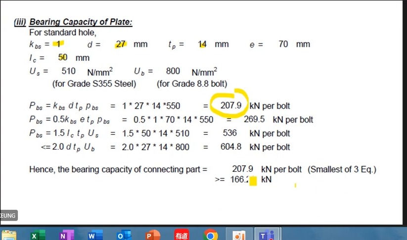
The bearing example uses M27, 14 mm plate, and . List all four capacities, especially keeping distinct from . The Q3 revision also explicitly divides total 200 kN by 2 to obtain 100 kN per side, consistent with the 26 September correction.
Complete worked examples in this unit: 850 kN lap weld: effective and provided lengths (Lap Weld) · M27 plate bearing: calculate all four bounds (Four Bearing Limits)
Eccentric weld groups: shear, torsion and resultant
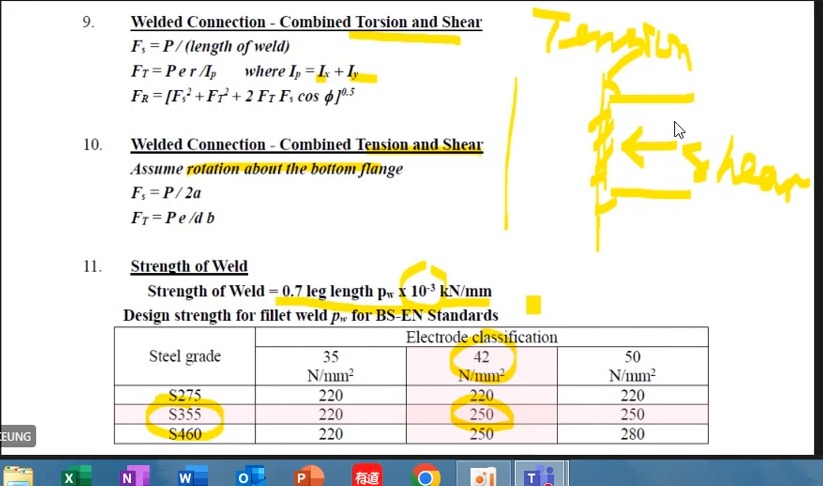
For in-plane eccentric weld groups, direct shear is distributed over total effective length . The force per unit length from is proportional to distance from the group centre.
Combine components vectorially rather than adding their magnitudes directly. For S355 with the course Class 42 electrode, the table gives .
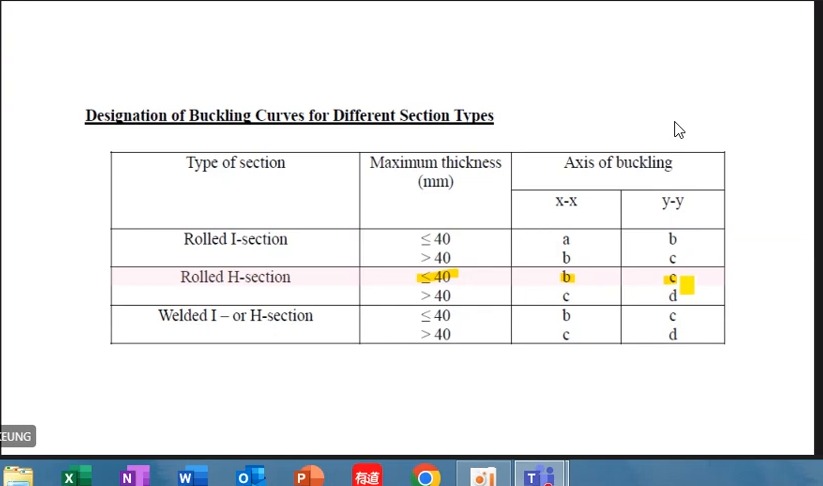
Buckling curves: match manufacture, thickness and axis
For example, the displayed rolled H-section with maximum thickness ≤40 mm uses curve b about and c about ; thickness >40 mm changes these to c and d.
Record the curve before reading . Slenderness alone does not define a unique compressive strength .
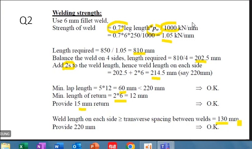
850 kN lap weld: effective to actual length
With , 6 mm legs give . Required total effective length is approximately 809.5 mm, rounded to 810 mm in class.
Four equal lines need about 202.5 mm each. Add to give 214.5 mm and adopt 220 mm. Also check minimum lap and end returns.
- The course minimum lap is 5×12=60 mm, below the provided 220 mm.
- Minimum end return is 2×6=12 mm; the course provides 15 mm.
- The longitudinal welds are 130 mm apart transversely. The provided 220 mm length also satisfies the corresponding requirement here.
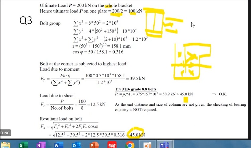
How to read this image: Check the squared-distance sum, maximum , 45 kN resultant and M16 resistance in sequence. The page also states that bearing data are not supplied.
Allocate angle weld lengths by centroid equilibrium
Connection width is 65 mm, giving 44.6 mm to the other side. Distribute the required 167 mm total effective length by moment equilibrium.
Side : 167×44.6/65≈115 mm; add 12 and adopt 130 mm. Side : about 52 mm; add 12 and adopt 65 mm. Provide 15 mm end returns.
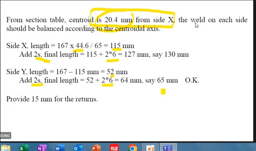
Plate-bearing example: minimum of four candidates
Given standard holes , , , and ; , and .
Candidates are 207.9, 269.5, 535.5 and 604.8 kN per bolt. Use 207.9. Displayed demand is about 166.7 kN per bolt, so this check passes.
850 kN lap weld: effective and provided lengths (Lap Weld)
A main plate is lapped to two cover plates with four 6 mm fillet welds and must pass on an ultimate tension of 850 kN. Find the weld length each run needs, confirm that the 220 mm provided is enough, and check that the main plate and cover plates are not pulled apart.
Solution Route: Resistance per millimetre→total effective length →divide among four lines→end allowance→actual selected length→detailing checks.
M27 plate bearing: calculate all four bounds (Four Bearing Limits)
One M27 bolt bears on a 14 mm plate. The end distance is 70 mm, the clear distance between holes is 50 mm, and the demand is about 166.7 kN per bolt. Work out the four bearing limits of the plate and compare the smallest with the demand.
Solution Route: Substitute into four expressions separately→compare in consistent units→take the minimum→compare with per-bolt demand.
Assignment beams and columns: match formulas to the problem (Assignment Checks)
What this unit is for: The assignment beams and columns use formulas already learnt, but each question has its own section and numbers; this unit matches every value to the question it belongs to.
Picture it this way: Beam: fix from the flange thickness first, then find , and only then compare the width-to-thickness ratios. Column: write each term as demand divided by capacity, with the amplification factor and m both on the demand, then add the three ratios and compare with 1. One length passing says nothing about another length.
Prerequisites: Will the plate buckle before its material strength is fully mobilised? (Section Classification) · Why a beam moves sideways and twists (Lateral-torsional Buckling) · Combined axial force and bending (Interaction Checks)
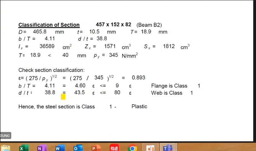
The B2 classification table uses and , unlike some earlier thinner beams with . Select strength before and or comparisons. Do not choose strength to obtain a desired class.
The added BC LTB page shows , , , and . This is another assignment beam with and demand 870.23, not the earlier B3 with .
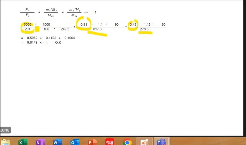
The later column interaction uses 3000 kN, and , totalling about 0.815. The recalculation below places both amplification and m factors on the demand side. This loading matches the final exercise on 31 October.
Another answer page uses 4310 kN and 305×305×158 UC: section utilisation 0.6215+0.0397+0.0617=0.7229≤1; LTB , and .
Complete worked examples in this unit: Column interaction revision: where each ratio comes from (Column Interaction Review)
B2 classification: thickness determines
The screen gives , and , with and .
and . Both are Class 1 for this bending condition.
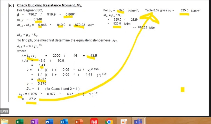
How to read this image: Identify and first, then demand 870.23 and resistance 920.8. Keep it separate from the earlier B3.
Column interaction: pair each demand with its resistance
The axial term uses and . Moment terms use and , with amplification factors 1.1 and 1.15 respectively.
The three displayed terms are about 0.5982, 0.1102 and 0.1064, totalling 0.8149≤1. This expression passes.
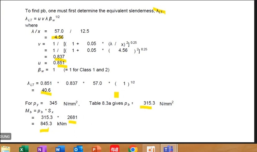
How to read this image: , and ; use for Classes 1/2.
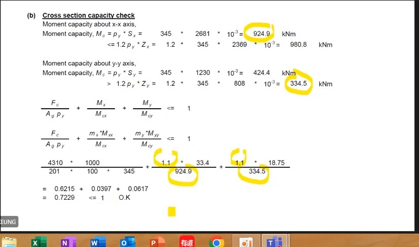
How to read this image: 4310/(201×100×345/1000)=0.6215; 1.1×33.4/924.9=0.0397; 1.1×18.75/334.5=0.0617.
Column interaction revision: where each ratio comes from (Column Interaction Review)
A 305×305×158 UC column carries 3000 kN of compression with moments of 90 kNm in the direction and 60 kNm in the direction. Recalculate the three ratios of the member interaction check one by one and see whether they add up to less than 1.
Solution Route: Calculate →amplify each directional demand→apply moment factors→divide by resistance→add.
Two floor beams: coexisting shear and independent SLS calculations (Beam Revision)
What this unit is for: Whether the moment capacity must be reduced depends on the shear at the place of maximum moment; this unit revises this point and deflection with two beam questions.
Picture it this way: Every position along a beam has its own pair of shear and moment. When bending is checked, the shear used for the judgement is the one at the place of maximum moment, not the largest shear from somewhere else. Deflection is worked out separately with everyday loads.
Prerequisites: Internal shear force and bending moment in a beam (Shear Force and Bending Moment) · Excessive bending deformation versus insufficient resistance (Deflection) · Use units to identify what you are calculating (Units and Dimensions)
The first has a 6 m span and 47.25 kN SLS point load; the second 8 m and 45 kN. Both use central-point-load deflection , but differs and span cubed magnifies the difference.
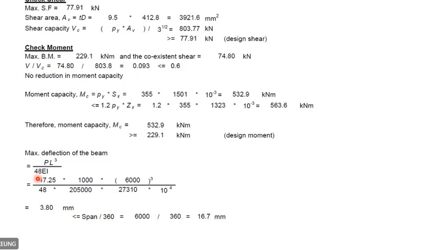
Maximum shear checks overall shear resistance . Shear coexisting at maximum moment determines high-shear reduction there. Different positions can have different values. The lecturer deliberately lists 77.91 and 74.80; they are not arbitrary rounding alternatives.
The problems differ in span , loading and . Select the correct ULS and SLS loads, then state units for every quantity.
Complete worked examples in this unit: 6 m revision beam: coexisting shear and deflection (Coexistent Shear) · 8 m revision beam: resistance and deformation again (Beam Check Practice)
Beam example: verify low shear and deflection separately
Here and maximum shear is 77.91 kN. At maximum moment 229.1 kNm, coexisting shear is 74.80 kN, giving . No high-shear reduction is needed.
Bending resistance exceeds 229.1. At SLS, central load 47.25 kN, and give deflection about 3.80 mm<16.7 mm.
Another floor-beam problem: strength and SLS use different values
The solution gives and . Coexisting shear ratio is about 0.10, allowing unreduced bending resistance .
. Unfactored over 8 m with gives deflection about 6.32 mm<22.2 mm.
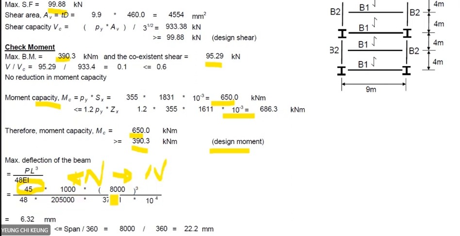
6 m revision beam: coexisting shear and deflection (Coexistent Shear)
A 6 m beam uses a 406×178×74 UB in S355. The largest shear is 77.91 kN, the largest moment is 229.1 kNm with a shear of 74.80 kN at that point, and the imposed midspan point load is 47.25 kN. Check shear, moment and deflection.
Solution Route: Overall shear→low shear at maximum moment→bending→unfactored deflection .
8 m revision beam: resistance and deformation again (Beam Check Practice)
A beam spanning 8000 mm uses a 457×191×82 UB in S355. The design moment is 390.3 kNm and the imposed midspan point load is 45 kN. Find the shear and moment capacities and check the deflection.
Solution Route: →→low-shear condition→→deflection and limit.
Past-paper connections and columns: restate new data (Past-paper Data)
What this unit is for: The new splice and column questions have entirely different numbers; this unit lists the data afresh and shows that the moment capacity in each direction is the smaller of two candidate values.
Picture it this way: For the column, copy the signed end moments for each direction, and take the larger one times the amplification factor as the demand. Each direction has two candidate moment capacities. Like a lorry that must pass under two bridges, the lower bridge sets the height allowed, so the smaller value is used.
Prerequisites: Several failure paths in a bolted connection (Bolted Connections) · Combined axial force and bending (Interaction Checks) · Why the position of a force matters (Moment and Eccentricity)
The past-paper splice gives 1200 kN, a 20 mm main plate, 14 mm covers, M27 bolts and 30 mm holes. Do not automatically combine this with the earlier bearing example. Read end and hole spacing from this new drawing.
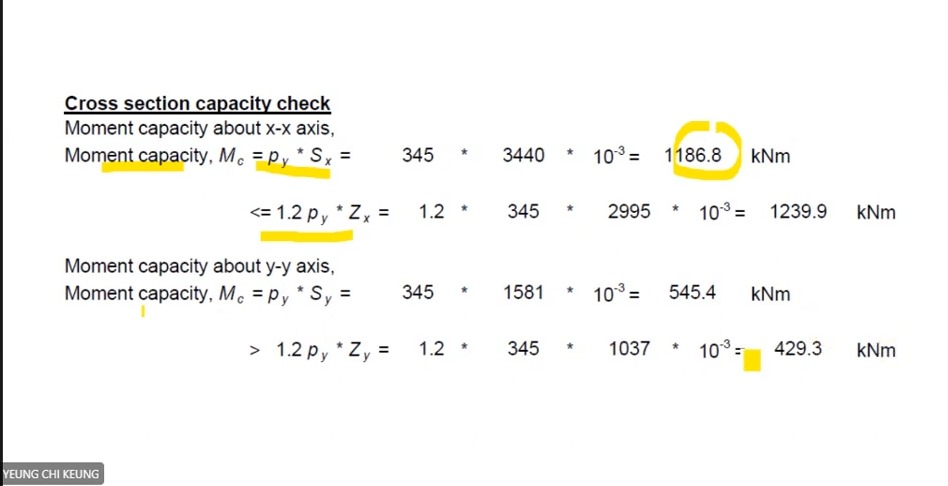
The 3500 kN column has signed moments about both axes and amplification 1.1. Governing demands are and ; section resistances are 1186.8 and 429.3 kNm. The weak-axis 1.2-times-elastic cap governs, so do not select the larger 545.4.
Another eccentric column has 3000 kN at its centre and 380, 240 and 350 kN on separate lines of action, with equal-stiffness upper/lower segments. This is a new problem: total axial force , take moments about both axes, then distribute. The lecturer does not complete capacity or the final verdict.
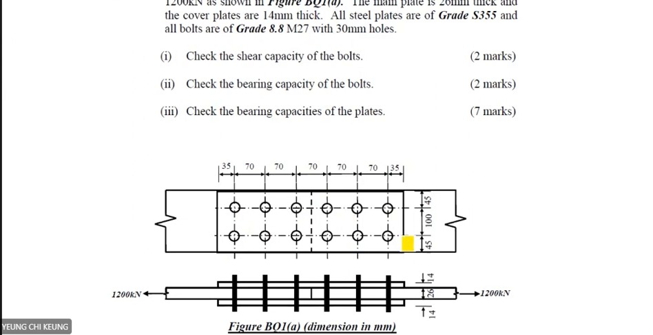
How to read this image: Read the new 20/14 mm thicknesses, 30 mm holes and dimensions such as 35/70. Do not borrow another problem's end distance.
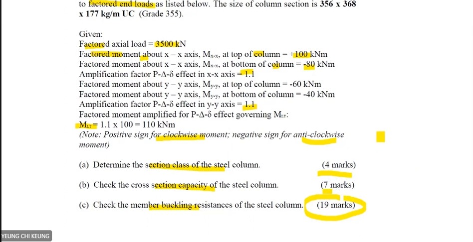
How to read this image: Retain all end signs. Record amplified governing values 110 and 66 separately from lookup data.
3500 kN column: list end moments separately
Axial force is 3500 kN; end moments +100/−80 kNm and end moments −60/−40 kNm. Both amplification factors are 1.1; .
The question asks for classification, section capacity and then member buckling. End-moment signs determine diagrams and factors; do not retain only maximum magnitudes and discard signs.
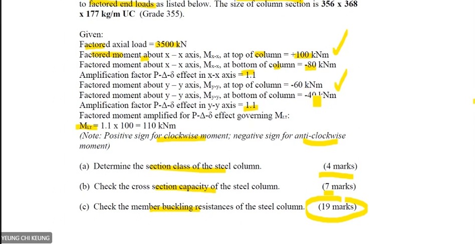
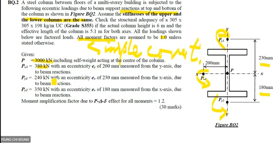
How to read this image: Distinguish central from eccentric loads before taking moments. This is not the previous 3500 kN problem.
3500 kN column: weak-axis elastic cap governs
. About , plastic resistance 1186.8 kNm is below the 1.2-times-elastic value 1239.9; use 1186.8.
About , plastic resistance 545.4 kNm exceeds the cap 429.3, so use 429.3. Combined axial/biaxial section checks and member buckling still follow.
LTB counterexample and segment restraints: Class 1 still needs stability (Stability Review)
What this unit is for: Class 1 only means the thin plates of the section will not wrinkle first; this unit uses a counter-example to show the whole beam can still buckle sideways.
Picture it this way: Classification looks closely at one plate at a time: the flange and web are thick enough not to wrinkle first. Lateral-torsional buckling steps back to look at the whole beam: the longer the unheld length, the more easily the compression flange drags the whole section sideways. Passing the first still leaves the second to be calculated with .
Prerequisites: Why a beam moves sideways and twists (Lateral-torsional Buckling) · Will the plate buckle before its material strength is fully mobilised? (Section Classification)
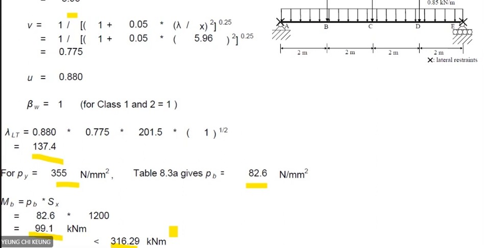
The lecturer shows a Class 1 beam with LTB resistance only 99.12 kNm. Class 1 describes local plates' ability to develop plasticity; it does not prevent sideways instability of the whole beam. Compare these local and global shapes in the foundation diagrams.
Convert to , read , then multiply by to obtain 99.12. This is clearly inadequate against 316.29. Do not replace with because material strength is high.
A later assignment BC segment has 2 m restraint length, , and , giving against 492.48 and passing. These are different problems and restraint conditions, not a correction from 99 to 762.
LTB counterexample: even Class 1 can fail
Ordinary slenderness is . With , and , . The table gives .
gives , below the displayed design demand 316.29 kNm. This LTB check fails.
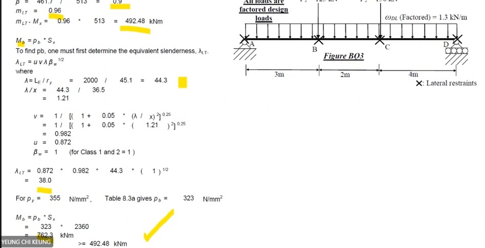
How to read this image: Locate restraints , , and and this segment's , then read , and 762.3>492.48.
Final deflection problem: use units to check yourself (Deflection and Units)
What this unit is for: The deflection formula mixes force, length and a section property, and mixed units throw the answer far off; this unit uses a point-load question to put everything in the same units.
Picture it this way: The span is multiplied together three times in the formula, so one slip between metres and millimetres throws the answer off many times over. Put every force in N and every length in mm, and the result comes out in mm, ready to compare with the limit of span divided by 360.
Prerequisites: Excessive bending deformation versus insufficient resistance (Deflection) · Use units to identify what you are calculating (Units and Dimensions)
The last problem uses 70 kN, 7 m and . Convert consistently to 70000 N, 7000 mm and 87318×10000 mm⁴; remains 205000 N/mm².
For a simply supported central point load, has units Nmm³ and has Nmm², leaving mm after division. This catches the error of putting 7 m directly into a millimetre-based calculation.
The result is about 2.79 mm, compared with 7000/360≈19.44 mm. Every course deflection example requires the correct model, units and SLS load. B1 uses UDL, unlike the point-load formula here.
Final deflection example: a 70 kN central point load
This separate problem uses , and . Convert to N and multiply by 10000 for mm⁴.
Deflection is approximately 2.79 mm, below . This serviceability check passes.