Worked Example

Example 5: biaxial checks for a non-sway-frame column (Biaxial Column)

Task: Record section and member checks separately and retain signed end moments.

Original question · Lecture notes Chapter 4, p. 36 (Example 5)
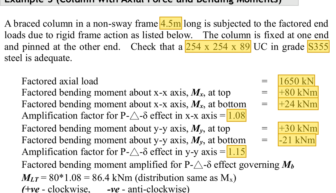
Original question with the given values boxed
Yellow boxes: values the question gives, the same values marked yellow in the Given table below.

The question in short: A 4.5 m column, 254×254×89 UC, is fixed at one end and pinned at the other. It carries 1650 kN of compression plus end moments about both axes. Decide whether the section is strong enough and whether the whole column buckles.

What differs from the previous example of this type: The previous example had compression only. This one also has moments about both the xx and yy axes, so interaction checks add the utilisation from compression and from each moment, with separate section and member checks.

GivenValue and Unit
Column4.5 m; fixed at one end, pinned at the other; 254×254×89 UC, S355
LoadingFc=1650 kN\htmlClass{given}{F_c=1650\ \mathrm{kN}}; xx end moments +80/+24; yy end moments +30/−21 kNm
Specified amplification1.08 about xx; 1.15 about yy
Material and section moduliT=17.3 mm\htmlClass{read}{T=17.3\ \mathrm{mm}}, py=345\htmlClass{read}{p_y=345}; Ag=113 cm2\htmlClass{read}{A_g=113\ \mathrm{cm^{2}}}; Sx=1224\htmlClass{read}{S_x=1224}, Zx=1096\htmlClass{read}{Z_x=1096}, Sy=575\htmlClass{read}{S_y=575}, Zy=379 cm3\htmlClass{read}{Z_y=379\ \mathrm{cm^{3}}}
Buckling datarx=112\htmlClass{read}{r_x=112}, ry=65.5 mm\htmlClass{read}{r_y=65.5\ \mathrm{mm}}; u=0.850\htmlClass{read}{u=0.850}, x=14.5\htmlClass{read}{x=14.5}

Yellow: values given in the question. The same values are marked where they are substituted in the steps below.
Orange box: values read directly from the Data File, the same values boxed orange in the lookup screenshots. A value interpolated between two table rows is a calculation, so it has no box.


Data file lookup · Data Page 11 · Universal Columns — Properties
254×254×89 UC: rx = 11.2 cm, ry = 6.55 cm, Zx = 1096, Zy = 379, Sx = 1224, Sy = 575 cm³, u = 0.850, x = 14.5, A = 113 cm².
254×254×89 UC: rx=11.2 cmr_x=11.2\ \mathrm{cm}, ry=6.55 cmr_y=6.55\ \mathrm{cm}, Zx=1096Z_x=1096, Zy=379Z_y=379, Sx=1224S_x=1224, Sy=575 cm3S_y=575\ \mathrm{cm^{3}}, u=0.850u=0.850, x=14.5x=14.5, A=113 cm2A=113\ \mathrm{cm^{2}}.Yellow: given parameter, row or columnOrange: value read from the table, boxed orange in the text too
Data file lookup · Data Page 11 · Universal Columns — Dimensions
254×254×89 UC: flange T = 17.3 mm.
254×254×89 UC: flange T=17.3 mmT=17.3\ \mathrm{mm}.Yellow: given parameter, row or columnOrange: value read from the table, boxed orange in the text too
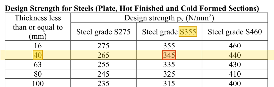
Data file lookup · Data Page 1 · Design strength pyp_y
T = 17.3 mm thick: the T ≤ 40 mm row, S355 column gives py = 345 N/mm².
T=17.3 mmT=17.3\ \mathrm{mm} thick: the T≤40 mmT\le40\ \mathrm{mm} row, S355 column gives py=345 N/mm2p_y=345\ \mathrm{N/mm^{2}}. How the grade and thickness choose this row →Yellow: given parameter, row or columnOrange: value read from the table, boxed orange in the text too
x-xy-yFlangeWebD: overall depthSchematic proportions; use the section table for actual dimensions
Supplementary schematic for understanding; not to scale.

Solution Route: Amplify demand→classification/section capacities→section interaction→effective length LeL_e/pc→moment factors→member interaction and LTB.

Load path · the stations the force passes through, in order

The column carries axial force and end moments about both axes together. The three actions use up the capacity together, so their three ratios are added, in three separate checks with different capacities.

  1. Axial force and amplified moments
    Fc=1650 kNF_c=1650\ \mathrm{kN}; Mx=86.4M_x=86.4, My=34.5 kNmM_y=34.5\ \mathrm{kNm}
  2. Cross-section check
    Sum 0.848Limit 1
  3. Member check 1 (buckling)
    Sum 0.949Limit 1
    closest to the limit
  4. Member check 2 (lateral-torsional buckling)
    Sum 0.935Limit 1
Red frame: the station closest to its limit. Each station links to the step that calculates it.
  1. Step 1 · Amplify demand

    Why this step: The given factors increase the moments to include the extra bending that appears once the compressed column deforms. For each axis the larger end moment is used, because that end is worked hardest.

    Apply the given factors to governing moments; do not add the two end moments.

    New symbols in this step
    • MxM_x, MyM_y, MLTM_{LT}: Two-axis and LTB governing moment demands; kNm
    • kxk_x, kyk_y, Mx1M_{x1}, My1M_{y1}: Amplification factors for the two axes; larger end moment before amplification, kNm
    Mx=kxMx1=1.08(80)=86.4,My=kyMy1=1.15(30)=34.5 kNmM_x=k_xM_{x1}={\htmlClass{given}{1.08}}({\htmlClass{given}{80}})=86.4,\quad M_y=k_yM_{y1}={\htmlClass{given}{1.15}}({\htmlClass{given}{30}})=34.5\ \mathrm{kNm}
    Mx=kxMx1=1.08(80)=86.4My=kyMy1=1.15(30)=34.5 kNm\begin{aligned}M_x&=k_xM_{x1}={\htmlClass{given}{1.08}}({\htmlClass{given}{80}})=86.4\\M_y&=k_yM_{y1}={\htmlClass{given}{1.15}}({\htmlClass{given}{30}})=34.5\ \mathrm{kNm}\end{aligned}

    ▶ The lecturer on this part: 31 October 00:24:38

  2. Step 2 · xx-axis section resistance

    Why this step: McxM_{cx} is the moment about the strong axis at which the steel across the whole section reaches pyp_y. It depends only on the section itself, not on the length of the column.

    For Class 1/2, plastic resistance is still capped at 1.2 times elastic resistance.

    New symbols in this step
    • AgA_g, pyp_y, pcp_c: Gross area mm²; yield and compression buckling strengths N/mm²
    • McxM_{cx}, McyM_{cy}, MbM_b: Corresponding bending resistances; kNm, with different section/member definitions
    Mcx=min⁡(pySx, 1.2pyZx)=min⁡(345(1224), 1.2(345)(1096))/1000=min⁡(422.28, 453.74)=422.28 kNm\begin{aligned}M_{cx}&=\min(p_yS_x,\ 1.2p_yZ_x)\\&=\min({\htmlClass{read}{345}}({\htmlClass{read}{1224}}),\ 1.2({\htmlClass{read}{345}})({\htmlClass{read}{1096}}))/1000\\&=\min(422.28,\ 453.74)=422.28\ \mathrm{kNm}\end{aligned}
    Mcx=min⁡(pySx, 1.2pyZx)=min⁡(345(1224), 1.2(345)(1096))/1000=min⁡(422.28, 453.74)=422.28 kNm\begin{aligned}M_{cx}&=\min(p_yS_x,\ 1.2p_yZ_x)\\&=\min({\htmlClass{read}{345}}({\htmlClass{read}{1224}}),\\&\quad \ 1.2({\htmlClass{read}{345}})({\htmlClass{read}{1096}}))/1000\\&=\min(422.28,\ 453.74)\\&=422.28\ \mathrm{kNm}\end{aligned}

    Units: pyp_y is in N/mm² and SxS_x or ZxZ_x in cm³. Since 1 cm³ = 1000 mm³, the product is in Nmm after multiplying by 1000. Changing Nmm to kNm divides by 1000000, a net division by 1000.

    ▶ The lecturer on this part: 31 October 00:29:38

  3. Step 3 · yy-axis section resistance

    Why this step: About the weak axis, SyS_y is much larger than ZyZ_y. The upper limit stops the steel from yielding under everyday loads, which would leave a permanent deformation.

    The cap governs the weak axis here.

    Mcy=min⁡(pySy, 1.2pyZy)=min⁡(345(575), 1.2(345)(379))/1000=min⁡(198.375, 156.906)=156.906 kNm\begin{aligned}M_{cy}&=\min(p_yS_y,\ 1.2p_yZ_y)\\&=\min({\htmlClass{read}{345}}({\htmlClass{read}{575}}),\ 1.2({\htmlClass{read}{345}})({\htmlClass{read}{379}}))/1000\\&=\min(198.375,\ 156.906)=156.906\ \mathrm{kNm}\end{aligned}
    Mcy=min⁡(pySy, 1.2pyZy)=min⁡(345(575), 1.2(345)(379))/1000=min⁡(198.375, 156.906)=156.906 kNm\begin{aligned}M_{cy}&=\min(p_yS_y,\ 1.2p_yZ_y)\\&=\min({\htmlClass{read}{345}}({\htmlClass{read}{575}}),\\&\quad \ 1.2({\htmlClass{read}{345}})({\htmlClass{read}{379}}))/1000\\&=\min(198.375,\ 156.906)\\&=156.906\ \mathrm{kNm}\end{aligned}

    Units: SyS_y and ZyZ_y are in cm³ and are multiplied by 1000 to give mm³. pyp_y times mm³ gives Nmm, and dividing by 1000000 gives kNm, so the formula divides by 1000.

  4. Step 4 · Section axial-compression resistance

    Why this step: This is the force that would crush the section itself, with all the steel at pyp_y and no bowing of the column considered. It is the capacity for the compression term in the section interaction check.

    Convert area to mm² before multiplying by pyp_y.

    Agpy=113(100)(345)/1000=3898.5 kNA_gp_y={\htmlClass{read}{113}}(100)({\htmlClass{read}{345}})/1000=3898.5\ \mathrm{kN}
    Agpy=113(100)(345)/1000=3898.5 kN\begin{aligned}A_gp_y&={\htmlClass{read}{113}}(100)({\htmlClass{read}{345}})/1000\\&=3898.5\ \mathrm{kN}\end{aligned}

    Units: AgA_g is multiplied by 100 to change cm² into mm². N/mm² times mm² gives N, and dividing by 1000 gives kN.

  5. Step 5 · Section interaction

    Why this step: Compression and the two moments all use the same steel at once. Each term is the share used by one action; if the three add up to no more than 1, the hardest-worked cross-section is not crushed.

    Every term is dimensionless; total is about 0.848.

    New symbols in this step
    • FcF_c, PcP_c: Design axial force and buckling compression resistance; kN
    • ηs\eta_s, η1\eta_1, η2\eta_2: Total utilisations for the section and two member expressions; dimensionless
    ηs=FcAgpy+MxMcx+MyMcy=1650/3898.5+86.4/422.28+34.5/156.906≈0.848\begin{aligned}\eta_s&=\frac{F_c}{A_gp_y}+\frac{M_x}{M_{cx}}+\frac{M_y}{M_{cy}}\\&={\htmlClass{given}{1650}}/3898.5+86.4/422.28+34.5/156.906\approx0.848\end{aligned}
    ηs=FcAgpy+MxMcx+MyMcy=1650/3898.5+86.4/422.28+34.5/156.906≈0.848\begin{aligned}\eta_s&=\frac{F_c}{A_gp_y}+\frac{M_x}{M_{cx}}+\frac{M_y}{M_{cy}}\\&={\htmlClass{given}{1650}}/3898.5\\&\quad +86.4/422.28\\&\quad +34.5/156.906\\&\approx0.848\end{aligned}

    Where the numbers come from: 3898.53898.5 from Step 4; 86.486.4 from Step 1; 422.28422.28 from Step 2; 34.534.5 from Step 1; 156.906156.906 from Step 3.

  6. Step 6 · Effective length

    Why this step: The fixed end stops the column from rotating there, so the part that bows is shorter, like a shorter pin-ended column. A shorter effective length makes buckling less likely.

    Fixed at one end and pinned at the other: the effective-length table in the lecture notes gives LE=0.85LL_E=0.85L.

    LE=0.85L=0.85(4500)=3825 mmL_E=0.85L=0.85({\htmlClass{given}{4500}})=3825\ \mathrm{mm}
    LE=0.85L=0.85(4500)=3825 mm\begin{aligned}L_E&=0.85L\\&=0.85({\htmlClass{given}{4500}})\\&=3825\ \mathrm{mm}\end{aligned}

    Units: The 4.5 m column height is multiplied by 1000 to give 4500 mm, so LEL_E is also in mm and can be divided directly by rxr_x and ryr_y in mm.

    ▶ The lecturer on this part: 31 October 00:34:56

  7. Step 7 · Two-axis slenderness and curves

    Why this step: With the same effective length, the smaller ryr_y makes the yy axis more slender and its pcp_c lower, so the column would bow about the weak axis first. PcP_c is the force it can carry before that happens.

    Use curve b (Table 8.8(b)) about xx and curve c (Table 8.8(c)) about yy, interpolating each in the py=345p_y=345 column; the smaller value, 246, governs.

    New symbols in this step
    • LeL_e, rxr_x, ryr_y, λ\lambda: Effective length and radius of gyration mm; dimensionless slenderness
    λx=LE/rx=3825/112≈34.2pcx=325+34.2−3035−30(318−325)≈319.1 N/mm2λy=LE/ry=3825/65.5≈58.4pcy=247+58.4−5860−58(241−247)≈245.8→246 N/mm2Pc=pcAg=246(113)(100)/1000=2779.8 kN\begin{aligned}\lambda_x&=L_E/r_x=3825/{\htmlClass{read}{112}}\approx34.2\\p_{cx}&={\htmlClass{read}{325}}+\frac{34.2-{\htmlClass{given}{30}}}{{\htmlClass{given}{35}}-{\htmlClass{given}{30}}}({\htmlClass{read}{318}}-{\htmlClass{read}{325}})\approx319.1\ \mathrm{N/mm^2}\\\lambda_y&=L_E/r_y=3825/{\htmlClass{read}{65.5}}\approx58.4\\p_{cy}&={\htmlClass{read}{247}}+\frac{58.4-{\htmlClass{given}{58}}}{{\htmlClass{given}{60}}-{\htmlClass{given}{58}}}({\htmlClass{read}{241}}-{\htmlClass{read}{247}})\approx245.8\to246\ \mathrm{N/mm^2}\\P_c&=p_cA_g=246({\htmlClass{read}{113}})(100)/1000=2779.8\ \mathrm{kN}\end{aligned}
    λx=LE/rx=3825/112≈34.2pcx=325+34.2−3035−30(318−325)≈319.1 N/mm2λy=LE/ry=3825/65.5≈58.4pcy=247+58.4−5860−58(241−247)≈245.8→246 N/mm2Pc=pcAg=246(113)(100)/1000=2779.8 kN\begin{aligned}\lambda_x&=L_E/r_x=3825/{\htmlClass{read}{112}}\approx34.2\\p_{cx}&={\htmlClass{read}{325}}+\frac{34.2-{\htmlClass{given}{30}}}{{\htmlClass{given}{35}}-{\htmlClass{given}{30}}}({\htmlClass{read}{318}}-{\htmlClass{read}{325}})\\&\approx319.1\ \mathrm{N/mm^2}\\\lambda_y&=L_E/r_y=3825/{\htmlClass{read}{65.5}}\approx58.4\\p_{cy}&={\htmlClass{read}{247}}+\frac{58.4-{\htmlClass{given}{58}}}{{\htmlClass{given}{60}}-{\htmlClass{given}{58}}}({\htmlClass{read}{241}}-{\htmlClass{read}{247}})\\&\approx245.8\to246\ \mathrm{N/mm^2}\\P_c&=p_cA_g\\&=246({\htmlClass{read}{113}})(100)/1000\\&=2779.8\ \mathrm{kN}\end{aligned}

    Where the numbers come from: 38253825 from Step 6.

    Units: AgA_g of 113 cm² is multiplied by 100 to change it into mm². pcp_c in N/mm² times mm² gives N, and dividing by 1000 gives kN. λ\lambda is mm divided by mm and has no unit.

    Data file lookup · Data Page 7 · Table 8.7 Buckling curves
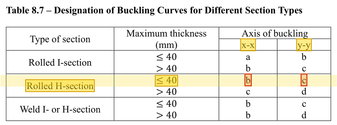
    Rolled H-section with thickness ≤ 40 mm: use curve b about the x-x axis and curve c about the y-y axis.
    Rolled H-section with thickness ≤ 40 mm: use curve b about the x-xx\text{-}x axis and curve c about the y-yy\text{-}y axis.Yellow: given parameter, row or columnOrange: value read from the table, boxed orange in the text too
    Data file lookup · Data Page 8 · Table 8.8(b)
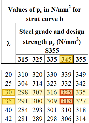
    Table 8.8(b) (x axis, curve b), py = 345 column: λ = 30 → 325 and λ = 35 → 318 N/mm²; interpolating at λx = 34.2 gives pc ≈ 319 N/mm².
    Table 8.8(b) (xx axis, curve b), py=345p_y=345 column: λ=30\lambda=30 → 325 and λ=35\lambda=35 → 318 N/mm²; interpolating at λx=34.2\lambda_{x}=34.2 gives pc≈319 N/mm2p_c\approx319\ \mathrm{N/mm^{2}}.Yellow: given parameter, row or columnOrange: value read from the table, boxed orange in the text too
    Data file lookup · Data Page 8 · Table 8.8(c)
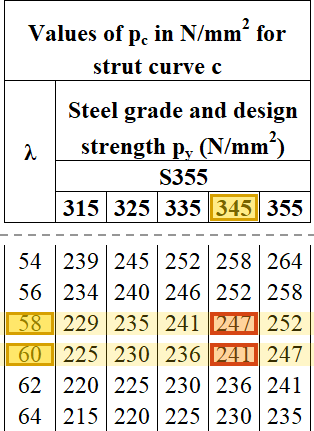
    Table 8.8(c) (y axis, curve c), py = 345 column: λ = 58 → 247 and λ = 60 → 241 N/mm²; interpolating at λy = 58.4 gives pc ≈ 246 N/mm².
    Table 8.8(c) (yy axis, curve c), py=345p_y=345 column: λ=58\lambda=58 → 247 and λ=60\lambda=60 → 241 N/mm²; interpolating at λy=58.4\lambda_{y}=58.4 gives pc≈246 N/mm2p_c\approx246\ \mathrm{N/mm^{2}}.Yellow: given parameter, row or columnOrange: value read from the table, boxed orange in the text too
  8. Step 8 · Moment-diagram factors

    Why this step: The moment changes along the column, so the largest moment does not act over the whole length. When the end moments bend the column into an SS shape, m is small; when they bend it into a single bow, m is larger.

    The course convention gives βx=−0.3\beta_{x}=-0.3 and βy=0.7\beta_{y}=0.7, then mx=0.54m_x=0.54 and my=0.88m_y=0.88. Do not mechanically divide the signed question values.

    New symbols in this step
    • mxm_x, mym_y, mLTm_{LT}: Equivalent moment-distribution factors; dimensionless
    βx=−24/80=−0.3 ⇒ mx=0.54,βy=21/30=0.7 ⇒ my=0.88\beta_x=-{\htmlClass{given}{24}}/{\htmlClass{given}{80}}=-0.3\ \Rightarrow\ m_x={\htmlClass{read}{0.54}},\qquad\beta_y={\htmlClass{given}{21}}/{\htmlClass{given}{30}}=0.7\ \Rightarrow\ m_y={\htmlClass{read}{0.88}}
    βx=−24/80=−0.3 ⇒ mx=0.54βy=21/30=0.7 ⇒ my=0.88\begin{aligned}\beta_x&=-{\htmlClass{given}{24}}/{\htmlClass{given}{80}}=-0.3\ \Rightarrow\ m_x={\htmlClass{read}{0.54}}\\\beta_y&={\htmlClass{given}{21}}/{\htmlClass{given}{30}}=0.7\ \Rightarrow\ m_y={\htmlClass{read}{0.88}}\end{aligned}
    Data file lookup · Data Page 7 · Table 8.9
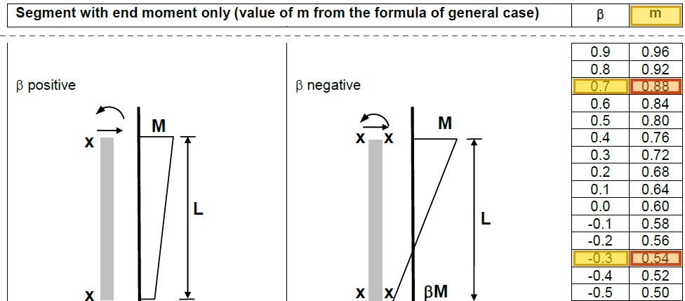
    Table 8.9: βy = 0.7 → my = 0.88; βx = −0.3 → mx = 0.54.
    Table 8.9: βy=0.7\beta_{y}=0.7 → my=0.88m_y=0.88; βx=−0.3\beta_{x}=-0.3 → mx=0.54m_x=0.54.Yellow: given parameter, row or columnOrange: value read from the table, boxed orange in the text too
  9. Step 9 · Elastic capacities for member checks

    Why this step: pyZp_yZ is the moment at which the outermost steel just reaches pyp_y, a more cautious value than the plastic capacity. It is the denominator when the whole column is checked for buckling.

    Use pyZp_yZ here, not the plastic capacities from the section check.

    Mcx,e=pyZx=345(1096)/1000=378.12 kNmMcy,e=pyZy=345(379)/1000=130.755 kNm\begin{aligned}M_{cx,e}&=p_yZ_x={\htmlClass{read}{345}}({\htmlClass{read}{1096}})/1000=378.12\ \mathrm{kNm}\\M_{cy,e}&=p_yZ_y={\htmlClass{read}{345}}({\htmlClass{read}{379}})/1000=130.755\ \mathrm{kNm}\end{aligned}
    Mcx,e=pyZx=345(1096)/1000=378.12 kNmMcy,e=pyZy=345(379)/1000=130.755 kNm\begin{aligned}M_{cx,e}&=p_yZ_x\\&={\htmlClass{read}{345}}({\htmlClass{read}{1096}})/1000\\&=378.12\ \mathrm{kNm}\\M_{cy,e}&=p_yZ_y\\&={\htmlClass{read}{345}}({\htmlClass{read}{379}})/1000\\&=130.755\ \mathrm{kNm}\end{aligned}

    Units: ZxZ_x and ZyZ_y are in cm³ and are multiplied by 1000 to give mm³. N/mm² times mm³ gives Nmm, and dividing by 1000000 gives kNm. Together this is a division by 1000.

    ▶ The lecturer on this part: 31 October 00:37:29

  10. Step 10 · First member check

    Why this step: This check asks whether the whole column, under compression and both moments together, bows out and buckles. The compression term uses PcP_c, so it is stricter than the section check.

    Recalculation with approximate parameters totals about 0.949.

    η1=FcPc+mxMxpyZx+myMypyZy=1650/2779.8+0.54(86.4)/378.12+0.88(34.5)/130.755≈0.949\begin{aligned}\eta_1&=\frac{F_c}{P_c}+\frac{m_xM_x}{p_yZ_x}+\frac{m_yM_y}{p_yZ_y}\\&={\htmlClass{given}{1650}}/2779.8+{\htmlClass{read}{0.54}}(86.4)/378.12+{\htmlClass{read}{0.88}}(34.5)/130.755\approx0.949\end{aligned}
    η1=FcPc+mxMxpyZx+myMypyZy=1650/2779.8+0.54(86.4)/378.12+0.88(34.5)/130.755≈0.949\begin{aligned}\eta_1&=\frac{F_c}{P_c}+\frac{m_xM_x}{p_yZ_x}+\frac{m_yM_y}{p_yZ_y}\\&={\htmlClass{given}{1650}}/2779.8\\&\quad +{\htmlClass{read}{0.54}}(86.4)/378.12\\&\quad +{\htmlClass{read}{0.88}}(34.5)/130.755\\&\approx0.949\end{aligned}

    Where the numbers come from: 2779.82779.8 from Step 7; 86.486.4 from Step 1; 378.12378.12 from Step 9; 34.534.5 from Step 1; 130.755130.755 from Step 9.

  11. Step 11 · LTB route

    Why this step: The moment about the strong axis compresses one flange, which can move sideways and make the column twist. The second member check guards against this by using MbM_b as the capacity in the xx-axis term.

    From λ\lambda, uu and xx find vv and λLT≈42.8\lambda_{LT}\approx42.8, interpolate pb≈308.6p_b\approx308.6 in the py=345p_y=345 column of Table 8.3a, then Mb≈377.7 kNmM_b\approx377.7\ \mathrm{kNm}; mLT=0.48m_{LT}=0.48 for β=−0.3\beta=-0.3. The second member check gives about 0.935.

    v=[1+0.05(58.4/14.5)2]−1/4≈0.862λLT=uvλ=0.850(0.862)(58.4)≈42.8pb=317+42.8−4045−40(302−317)≈308.6 N/mm2Mb=pbSx=308.6(1224)/1000≈377.7 kNmη2=FcPc+mLTMLTMb+myMypyZy≈1650/2779.8+0.48(86.4)/377.7+0.88(34.5)/130.755≈0.935\begin{aligned}v&=\left[1+0.05(58.4/{\htmlClass{read}{14.5}})^2\right]^{-1/4}\approx0.862\\\lambda_{LT}&=uv\lambda={\htmlClass{read}{0.850}}(0.862)(58.4)\approx42.8\\p_b&={\htmlClass{read}{317}}+\frac{42.8-{\htmlClass{given}{40}}}{{\htmlClass{given}{45}}-{\htmlClass{given}{40}}}({\htmlClass{read}{302}}-{\htmlClass{read}{317}})\approx308.6\ \mathrm{N/mm^2}\\M_b&=p_bS_x=308.6({\htmlClass{read}{1224}})/1000\approx377.7\ \mathrm{kNm}\\\eta_2&=\frac{F_c}{P_c}+\frac{m_{LT}M_{LT}}{M_b}+\frac{m_yM_y}{p_yZ_y}\\&\approx{\htmlClass{given}{1650}}/2779.8+{\htmlClass{read}{0.48}}(86.4)/377.7+{\htmlClass{read}{0.88}}(34.5)/130.755\approx0.935\end{aligned}
    v=[1+0.05(58.4/14.5)2]−1/4≈0.862λLT=uvλ=0.850(0.862)(58.4)≈42.8pb=317+42.8−4045−40(302−317)≈308.6 N/mm2Mb=pbSx=308.6(1224)/1000≈377.7 kNmη2=FcPc+mLTMLTMb+myMypyZy≈1650/2779.8+0.48(86.4)/377.7+0.88(34.5)/130.755≈0.935\begin{aligned}v&=\left[1+0.05(58.4/{\htmlClass{read}{14.5}})^2\right]^{-1/4}\\&\approx0.862\\\lambda_{LT}&=uv\lambda\\&={\htmlClass{read}{0.850}}(0.862)(58.4)\\&\approx42.8\\p_b&={\htmlClass{read}{317}}+\frac{42.8-{\htmlClass{given}{40}}}{{\htmlClass{given}{45}}-{\htmlClass{given}{40}}}({\htmlClass{read}{302}}-{\htmlClass{read}{317}})\\&\approx308.6\ \mathrm{N/mm^2}\\M_b&=p_bS_x\\&=308.6({\htmlClass{read}{1224}})/1000\\&\approx377.7\ \mathrm{kNm}\\\eta_2&=\frac{F_c}{P_c}+\frac{m_{LT}M_{LT}}{M_b}+\frac{m_yM_y}{p_yZ_y}\\&\approx{\htmlClass{given}{1650}}/2779.8\\&\quad +{\htmlClass{read}{0.48}}(86.4)/377.7\\&\quad +{\htmlClass{read}{0.88}}(34.5)/130.755\\&\approx0.935\end{aligned}

    Where the numbers come from: 58.458.4 from Step 7; 2779.82779.8 from Step 7; 86.486.4 from Step 1; 34.534.5 from Step 1; 130.755130.755 from Step 9.

    Units: In Mb=pbM_b=p_b SxS_x, SxS_x is in cm³ and is multiplied by 1000 to give mm³. N/mm² times mm³ gives Nmm, and dividing by 1000000 gives kNm, so only a division by 1000 remains.

    Data file lookup · Data Page 6 · Table 8.4a

    Table 8.4a: β = −0.3 → mLT = 0.48.
    Table 8.4a: β=−0.3\beta=-0.3 → mLT=0.48m_{LT}=0.48.Yellow: given parameter, row or columnOrange: value read from the table, boxed orange in the text too
    Data file lookup · Data Page 5 · Table 8.3a
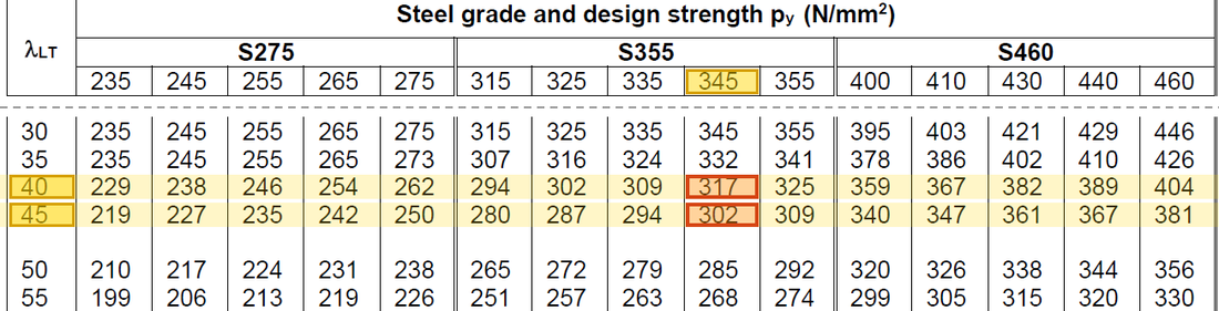
    Table 8.3a, py = 345 column: λLT = 40 → 317 and λLT = 45 → 302 N/mm²; interpolating at λLT = 42.8 gives pb ≈ 308.6 N/mm².
    Table 8.3a, py=345p_y=345 column: λLT=40\lambda_{LT}=40 → 317 and λLT=45\lambda_{LT}=45 → 302 N/mm²; interpolating at λLT=42.8\lambda_{LT}=42.8 gives pb≈308.6 N/mm2p_b\approx308.6\ \mathrm{N/mm^{2}}.Yellow: given parameter, row or columnOrange: value read from the table, boxed orange in the text too
    Load path · How the ratios add up
    Limit 1Cross-section0.4230.2050.22≈ 0.848Member 1 (buckling)0.5940.1230.232≈ 0.949Member 2 (LTB)0.5940.110.232≈ 0.935Axial termx-axis moment termy-axis moment term
    Each bar is one check: blue is the share used by the axial force, green and yellow the shares used by the moments about the two axes. Together they must not pass the red dashed line.

    ▶ The lecturer on this part: 31 October 00:40:00

Conclusion

With these parameters, the section and both member interactions are below 1. Their different totals reflect different failure modes; do not use the smallest to stand for all checks.

All the symbols of this example

SymbolsMeaning and Units
FcF_c, PcP_cDesign axial force and buckling compression resistance; kN
AgA_g, pyp_y, pcp_cGross area mm²; yield and compression buckling strengths N/mm²
LeL_e, rxr_x, ryr_y, λ\lambdaEffective length and radius of gyration mm; dimensionless slenderness
MxM_x, MyM_y, MLTM_{LT}Two-axis and LTB governing moment demands; kNm
SxS_x, SyS_y, ZxZ_x, ZyZ_yTwo-axis plastic/elastic moduli; convert the tabulated cm³
McxM_{cx}, McyM_{cy}, MbM_bCorresponding bending resistances; kNm, with different section/member definitions
mxm_x, mym_y, mLTm_{LT}Equivalent moment-distribution factors; dimensionless
ηs\eta_s, η1\eta_1, η2\eta_2Total utilisations for the section and two member expressions; dimensionless
kxk_x, kyk_y, Mx1M_{x1}, My1M_{y1}Amplification factors for the two axes; larger end moment before amplification, kNm

Video positions: 31 October 00:25:00 · 31 October 00:30:00 · 31 October 00:35:00 · 31 October 00:40:00

↑ Top