Worked Example

B2: the internal beam in the same floor (Interior Beam)

Task: Check the complete corrected dataset and recognise the loading difference between internal and edge beams.

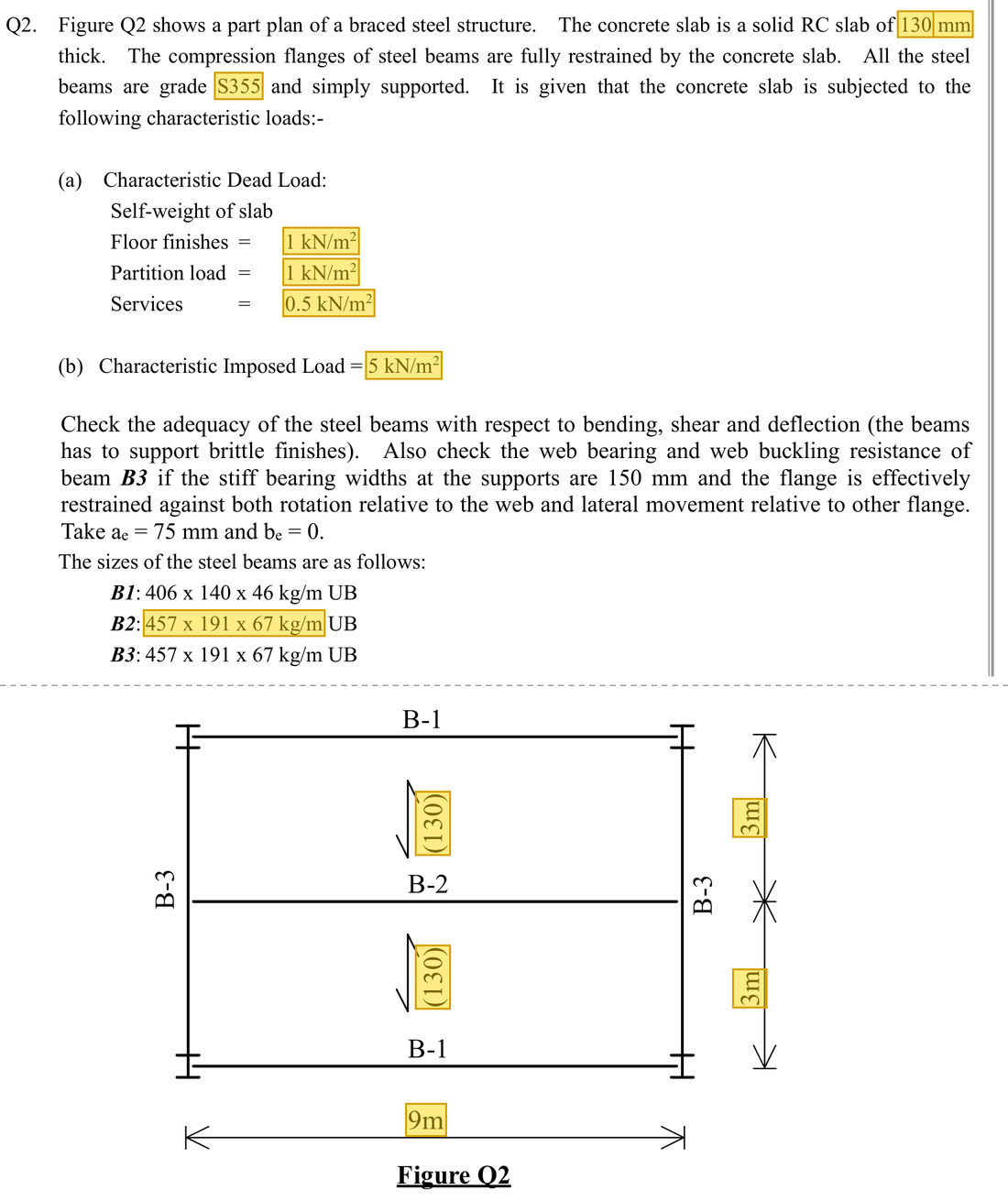
Original question · Lecture notes Chapter 3, p. 35–36 (Tutorial 3 Q2)
Original question with the given values boxed
Yellow boxes: values the question gives, the same values marked yellow in the Given table below.

The question in short: An interior beam in the same floor spans 9 m with a 3 m slab span on each side, a 130 mm slab and a 5 kN/m² imposed load. Decide whether a 457×191×67 UB in S355 passes for strength and deflection.

What differs from the previous example of this type: B1 is an edge beam carrying slab on one side only. B2 is in the middle with slab on both sides, so its load is about double and a larger section is used.

GivenValue and Unit
ModelSimply supported span 9 m; slab span 3 m on each side
Slab and dead area loadsSlab 130 mm thick; finishes 1, partitions 1, services 0.5 kN/m²
Imposed area load5 kN/m²
Section457×191×67 UB (67 kg/m), S355; D=453.4\htmlClass{read}{D=453.4}, t=8.5\htmlClass{read}{t=8.5}, T=12.7 mm\htmlClass{read}{T=12.7\ \mathrm{mm}}; b/T=7.48\htmlClass{read}{b/T=7.48}, d/t=48\htmlClass{read}{d/t=48}
Material and section modulipy=355\htmlClass{read}{p_y=355}; Sx=1471\htmlClass{read}{S_x=1471}, Zx=1296 cm3\htmlClass{read}{Z_x=1296\ \mathrm{cm^{3}}}; Ix=29380 cm4\htmlClass{read}{I_x=29380\ \mathrm{cm^{4}}}

Yellow: values given in the question. The same values are marked where they are substituted in the steps below.
Orange box: values read directly from the Data File, the same values boxed orange in the lookup screenshots. A value interpolated between two table rows is a calculation, so it has no box.
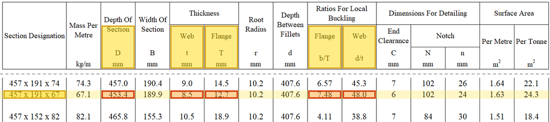
Data file lookup · Data Page 9 · Universal Beams — Dimensions
457×191×67 UB: D = 453.4 mm, t = 8.5 mm, T = 12.7 mm; b/T = 7.48, d/t = 48.0.
457×191×67 UB: D=453.4 mmD=453.4\ \mathrm{mm}, t=8.5 mmt=8.5\ \mathrm{mm}, T=12.7 mmT=12.7\ \mathrm{mm}; b/T=7.48b/T=7.48, d/t=48.0d/t=48.0.Yellow: given parameter, row or columnOrange: value read from the table, boxed orange in the text too
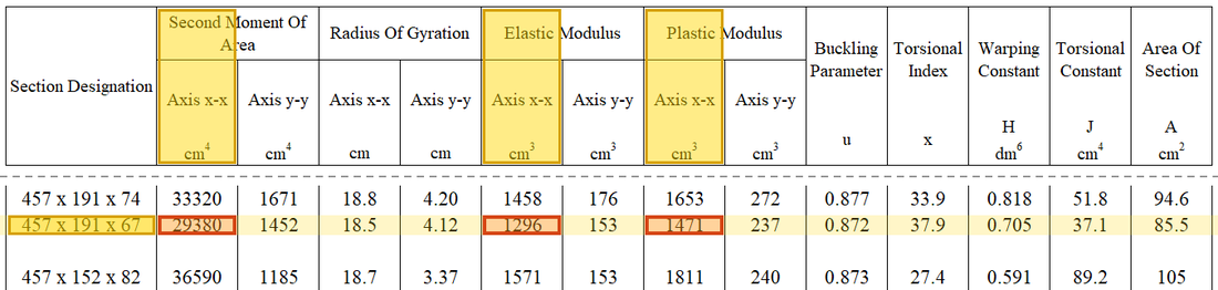
Data file lookup · Data Page 10 · Universal Beams — Properties
457×191×67 UB: Ix = 29380 cm⁴, Zx = 1296 cm³, Sx = 1471 cm³.
457×191×67 UB: Ix=29380 cm4I_x=29380\ \mathrm{cm^{4}}, Zx=1296 cm3Z_x=1296\ \mathrm{cm^{3}}, Sx=1471 cm3S_x=1471\ \mathrm{cm^{3}}.Yellow: given parameter, row or columnOrange: value read from the table, boxed orange in the text too
UDL w (kN/m)RA​RB​Span between supports, L
Supplementary schematic for understanding; not to scale.

Solution Route: Trace loading from both slab sides; cross-check internal actions; classify and compare shear and two bending candidates; list SLS separately.

Load path · the stations the force passes through, in order

B2 is an interior beam with slab on both sides, so its tributary width is twice that of B1. Its ends sit on B3, and its reactions become the load on B3.

  1. Area load on the slab
    Times the 3 m tributary width
  2. Line load on B2
    ULS: 48.64 kN/m
  3. B2 in bending (midspan)
    Demand 492.48 kNmCapacity 522.205 kNm
    Utilisation 0.94 · closest to the limit
  4. B2 in shear (supports)
    Demand 218.88 kNCapacity 789.89 kN
    Utilisation 0.28
  5. Deflection (imposed load)
    Demand 21.2762 mmCapacity 25 mm
    Utilisation 0.85
  6. Support reactions
    218.88 kN at each end, onto the midspan of B3
Red frame: the station closest to its limit. Each station links to the step that calculates it.
Load path · Floor plan: which part of the slab each beam carries
B1B1B2B3B3Column9 m3 m3 m6 m11Shaded: the slab B2 carries, 1.5 m on each side, so the tributary width is 3 m22Area load × 3 m gives the line load on B2: w = 48.64 kN/m at ULS33B2 has a 218.88 kN reaction at each end, onto the midspan of B3 (circles)Arrows: the direction the load travels (plan seen from above)
B2 is in the middle: the slab on each side gives it half its load, so the tributary width is 3 m and the line load is about twice that of B1. The ends of B2 sit on B3, not on columns.
  1. Step 1 · Tributary width

    Why this step: An interior beam has slab pressing down from both sides, so it looks after a wider strip than an edge beam and every floor load grows with it.

    B2 collects half a bay on each side, totalling 3 m. Do not copy B1's 1.5 m.

    New symbols in this step
    • hh, btribb_{trib}: Slab thickness, tributary width; m
    btrib=3/2+3/2=3 mb_{trib}={\htmlClass{given}{3}}/2+{\htmlClass{given}{3}}/2={\htmlClass{given}{3}}\ \mathrm{m}
  2. Step 2 · Permanent line load

    Why this step: Self-weight, slab and finishes all rest on the beam permanently. Adding them into one load per metre gives a figure the beam formulas can use.

    The beam self-weight of 67 kg/m is about 0.67 kN/m; the slab weight is the thickness times the unit weight 24 kN/m³ (the usual value the lecturer uses) times the 3 m tributary width btribb_{trib}; the three dead area loads qq are also multiplied by 3 m. After the correction in class, 17.53 is rounded up to 17.6 instead of the 9 left over from the worksheet.

    wsw=67(10)/1000=0.67,wslab=0.13(24)(3)=9.36 kN/mGk=0.67+9.36+(1+1+0.5)(3)=17.53→17.6 kN/m\begin{aligned}w_{sw}&={\htmlClass{given}{67}}(10)/1000=0.67,\quad w_{slab}={\htmlClass{given}{0.13}}(24)({\htmlClass{given}{3}})=9.36\ \mathrm{kN/m}\\G_k&=0.67+9.36+({\htmlClass{given}{1}}+{\htmlClass{given}{1}}+{\htmlClass{given}{0.5}})({\htmlClass{given}{3}})=17.53\to17.6\ \mathrm{kN/m}\end{aligned}
    wsw=67(10)/1000=0.67wslab=0.13(24)(3)=9.36 kN/mGk=0.67+9.36+(1+1+0.5)(3)=17.53→17.6 kN/m\begin{aligned}w_{sw}&={\htmlClass{given}{67}}(10)/1000=0.67\\w_{slab}&={\htmlClass{given}{0.13}}(24)({\htmlClass{given}{3}})=9.36\ \mathrm{kN/m}\\G_k&=0.67+9.36+({\htmlClass{given}{1}}+{\htmlClass{given}{1}}+{\htmlClass{given}{0.5}})({\htmlClass{given}{3}})\\&=17.53\to17.6\ \mathrm{kN/m}\end{aligned}

    Units: kg/m times 10 gives N/m, and dividing by 1000 gives kN/m (1 kN is 1000 N). The 130 mm slab is also written as 0.13 m first.

    ▶ The lecturer on this part: 17 October 01:04:59

  3. Step 3 · Imposed load and ULS

    Why this step: This is the load for the strength checks. Dead and imposed loads are each enlarged and then added, to represent the worst case the beam may meet.

    Only area loads qq need multiplication by tributary width btribb_{trib}. The permanent components listed here are already line loads ww.

    New symbols in this step
    • GkG_k, QkQ_k: Unfactored dead and imposed loads; kN/m or kN
    Qk=qkbtrib=5(3)=15 kN/mw=1.4Gk+1.6Qk=1.4(17.6)+1.6(15)=48.64 kN/m\begin{aligned}Q_k&=q_kb_{trib}={\htmlClass{given}{5}}({\htmlClass{given}{3}})=15\ \mathrm{kN/m}\\w&=1.4G_k+1.6Q_k=1.4(17.6)+1.6(15)=48.64\ \mathrm{kN/m}\end{aligned}
    Qk=qkbtrib=5(3)=15 kN/mw=1.4Gk+1.6Qk=1.4(17.6)+1.6(15)=48.64 kN/m\begin{aligned}Q_k&=q_kb_{trib}={\htmlClass{given}{5}}({\htmlClass{given}{3}})=15\ \mathrm{kN/m}\\w&=1.4G_k+1.6Q_k\\&=1.4(17.6)+1.6(15)\\&=48.64\ \mathrm{kN/m}\end{aligned}
  4. Step 4 · Reactions and maximum moment

    Why this step: This gives the largest shear at the ends and the largest moment at midspan. They are the demands for the shear and moment checks that follow.

    Use the same load and span LL to reproduce the corrected internal actions.

    New symbols in this step
    • MM, VV: Moment demand in kNm; shear demand in kN
    V=wL/2=48.64(9)/2=218.88 kNM=wL2/8=48.64(9)2/8=492.48 kNm\begin{aligned}V&=wL/2=48.64({\htmlClass{given}{9}})/2=218.88\ \mathrm{kN}\\M&=wL^2/8=48.64({\htmlClass{given}{9}})^2/8=492.48\ \mathrm{kNm}\end{aligned}
    V=wL/2=48.64(9)/2=218.88 kNM=wL2/8=48.64(9)2/8=492.48 kNm\begin{aligned}V&=wL/2\\&=48.64({\htmlClass{given}{9}})/2\\&=218.88\ \mathrm{kN}\\M&=wL^2/8\\&=48.64({\htmlClass{given}{9}})^2/8\\&=492.48\ \mathrm{kNm}\end{aligned}

    Where the numbers come from: 48.6448.64 from Step 3.

    Load path · Load, shear force and bending moment
    Loads and reactionsw = 48.64 kN/mRA​ = 218.88 kNRB​ = 218.88 kN9 mShear force diagram V (kN)218.88−218.88Bending moment diagram M (kNm): sagging moment drawn below the lineV = 0Mmax​ = 492.48 kNm
    The same model as B1 with a larger line load. The 218.88 kN reaction at each end is the point load at the midspan of B3 in the next example.

    ▶ The lecturer on this part: 17 October 01:04:00

  5. Step 5 · Material and classification

    Why this step: Thicker steel may have a lower design strength, so pyp_y is set from the flange thickness first. Then the flange and web are confirmed not to be so thin that they buckle locally first.

    T=12.7 mmT=12.7\ \mathrm{mm} gives py=355p_y=355 and ε≈0.8801\varepsilon\approx0.8801. For this bending row, b/T=7.48<9ε≈7.92b/T=7.48<9\varepsilon\approx7.92 and d/t=48<80ε≈70.41d/t=48<80\varepsilon\approx70.41, hence Class 1.

    New symbols in this step
    • DD, dd, tt, TT: Overall depth, classification web depth, web thickness and flange thickness; mm
    • pyp_y, pbp_b, EE: Design yield/bending buckling strength and elastic modulus; N/mm²
    ε=275/py=275/355≈0.8801b/T=7.48<9ε≈7.92,d/t=48<80ε≈70.41\begin{aligned}\varepsilon&=\sqrt{275/p_y}=\sqrt{275/{\htmlClass{read}{355}}}\approx0.8801\\b/T&={\htmlClass{read}{7.48}}<{\htmlClass{read}{9}}\varepsilon\approx7.92,\qquad d/t={\htmlClass{read}{48}}<{\htmlClass{read}{80}}\varepsilon\approx70.41\end{aligned}
    ε=275/py=275/355≈0.8801b/T=7.48<9ε≈7.92d/t=48<80ε≈70.41\begin{aligned}\varepsilon&=\sqrt{275/p_y}=\sqrt{275/{\htmlClass{read}{355}}}\approx0.8801\\b/T&={\htmlClass{read}{7.48}}<{\htmlClass{read}{9}}\varepsilon\approx7.92\\d/t&={\htmlClass{read}{48}}<{\htmlClass{read}{80}}\varepsilon\approx70.41\end{aligned}
    Data file lookup · Data Page 1 · Design strength pyp_y
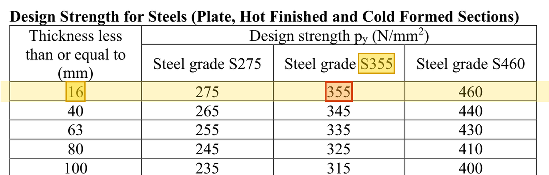
    Flange T = 12.7 mm thick: the T ≤ 16 mm row, S355 column gives py = 355 N/mm².
    Flange T=12.7 mmT=12.7\ \mathrm{mm} thick: the T≤16 mmT\le16\ \mathrm{mm} row, S355 column gives py=355 N/mm2p_y=355\ \mathrm{N/mm^{2}}. How the grade and thickness choose this row →Yellow: given parameter, row or columnOrange: value read from the table, boxed orange in the text too
    Data file lookup · Data Page 1 · Table 7.1 Limiting width-to-thickness ratios
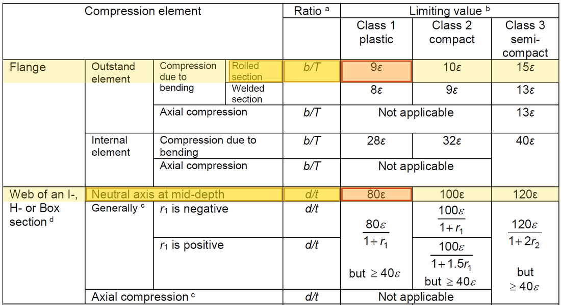
    Same table: with py = 355, ε ≈ 0.8801, 9ε ≈ 7.92 and 80ε ≈ 70.4; b/T = 7.48 and d/t = 48.0 are both within the Class 1 limits.
    Same table: with py=355p_y=355, ε≈0.8801\varepsilon\approx0.8801, 9ε ≈ 7.92 and 80ε ≈ 70.4; b/T=7.48b/T=7.48 and d/t=48.0d/t=48.0 are both within the Class 1 limits.Yellow: given parameter, row or columnOrange: value read from the table, boxed orange in the text too
  6. Step 6 · Web shear area

    Why this step: This is the web area available to resist shear. The larger it is, the harder it is for the beam end to fail in shear.

    Use tDtD for the rolled I-section.

    New symbols in this step
    Av=tD=8.5(453.4)=3853.9 mm2A_v=tD={\htmlClass{read}{8.5}}({\htmlClass{read}{453.4}})=3853.9\ \mathrm{mm^2}
  7. Step 7 · Shear resistance

    Why this step: This guards against the web shearing near the supports. A low enough ratio also means shear does not weaken the section's bending strength.

    Convert N to kN before comparing with 218.88, and also check low shear.

    New symbols in this step
    • McM_c, VcV_c, MbM_b: Section bending resistance in kNm, shear resistance in kN, LTB resistance in kNm
    Vc=pyAv/3=355(3853.9)/(3 1000)≈789.89 kNV/Vc=218.88/789.89≈0.277<0.6\begin{aligned}V_c&=p_yA_v/\sqrt3={\htmlClass{read}{355}}(3853.9)/(\sqrt3\,1000)\approx789.89\ \mathrm{kN}\\V/V_c&=218.88/789.89\approx0.277<0.6\end{aligned}
    Vc=pyAv/3=355(3853.9)/(3 1000)≈789.89 kNV/Vc=218.88/789.89≈0.277<0.6\begin{aligned}V_c&=p_yA_v/\sqrt3\\&={\htmlClass{read}{355}}(3853.9)/(\sqrt3\,1000)\\&\approx789.89\ \mathrm{kN}\\V/V_c&=218.88/789.89\\&\approx0.277\\&<0.6\end{aligned}

    Where the numbers come from: 3853.93853.9 from Step 6; 218.88218.88 from Step 4.

    Units: N/mm² times mm² gives N. Dividing by 1000 changes N into kN, because 1 kN is 1000 N.

  8. Step 8 · Bending candidates

    Why this step: This guards against the section yielding where the moment is greatest. The smaller of the two candidates is the moment capacity the section can really rely on.

    Convert SS and ZZ from cm³ and take the smaller candidate.

    Mc=min⁡(pySx, 1.2pyZx)=min⁡(355(1471), 1.2(355)(1296))/1000=min⁡(522.205, 552.096)=522.205 kNm\begin{aligned}M_c&=\min(p_yS_x,\ 1.2p_yZ_x)\\&=\min({\htmlClass{read}{355}}({\htmlClass{read}{1471}}),\ 1.2({\htmlClass{read}{355}})({\htmlClass{read}{1296}}))/1000\\&=\min(522.205,\ 552.096)=522.205\ \mathrm{kNm}\end{aligned}
    Mc=min⁡(pySx, 1.2pyZx)=min⁡(355(1471), 1.2(355)(1296))/1000=min⁡(522.205, 552.096)=522.205 kNm\begin{aligned}M_c&=\min(p_yS_x,\ 1.2p_yZ_x)\\&=\min({\htmlClass{read}{355}}({\htmlClass{read}{1471}}),\\&\quad \ 1.2({\htmlClass{read}{355}})({\htmlClass{read}{1296}}))/1000\\&=\min(522.205,\ 552.096)\\&=522.205\ \mathrm{kNm}\end{aligned}

    Units: N/mm² times cm³ gives 1000 Nmm (1 cm³ is 1000 mm³). 1 kNm is 1000000 Nmm, so overall the product only needs dividing by 1000.

    ▶ The lecturer on this part: 17 October 01:04:00

  9. Step 9 · Bending comparison

    Why this step: A utilisation very close to one means the section's bending strength is almost fully used, with little margin left.

    Demand 492.48 is relatively close to resistance; retain the identity of both values.

    ηM=M/Mc=492.48/522.205≈0.943<1\eta_M=M/M_c=492.48/522.205\approx0.943<1
    ηM=M/Mc=492.48/522.205≈0.943<1\begin{aligned}\eta_M&=M/M_c\\&=492.48/522.205\\&\approx0.943\\&<1\end{aligned}

    Where the numbers come from: 492.48492.48 from Step 4; 522.205522.205 from Step 8.

  10. Step 10 · Independent SLS check

    Why this step: Being strong enough does not mean the beam will not sag too much. This step uses the everyday imposed load to see whether the midspan sag stays within the limit.

    Use unfactored imposed line load ww 15 kN/m=15 N/mm, E=205000E=205000, L=9000L=9000 and I=29380×10000I=29380\times10000.

    New symbols in this step
    • LL, RAR_A, RBR_B: Span in m or mm; end reactions in kN
    • Δ\Delta, η\eta: Deflection mm; demand/resistance utilisation is dimensionless
    Δ=5wL4384EI=5(15)(9000)4384(205000)(29380×104)≈21.2762 mm<L/360=9000/360=25 mm\begin{aligned}\Delta&=\frac{5wL^4}{384EI}=\frac{5(15)({\htmlClass{given}{9000}})^4}{384({\htmlClass{read}{205000}})({\htmlClass{read}{29380}}\times10^4)}\approx21.2762\ \mathrm{mm}\\&<L/{\htmlClass{read}{360}}={\htmlClass{given}{9000}}/{\htmlClass{read}{360}}=25\ \mathrm{mm}\end{aligned}
    Δ=5wL4384EI=5(15)(9000)4384(205000)(29380×104)≈21.2762 mm<L/360=9000/360=25 mm\begin{aligned}\Delta&=\frac{5wL^4}{384EI}\\&=\frac{5(15)({\htmlClass{given}{9000}})^4}{384({\htmlClass{read}{205000}})({\htmlClass{read}{29380}}\times10^4)}\\&\approx21.2762\ \mathrm{mm}\\&<L/{\htmlClass{read}{360}}={\htmlClass{given}{9000}}/{\htmlClass{read}{360}}=25\ \mathrm{mm}\end{aligned}

    Where the numbers come from: 1515 from Step 3.

    Units: IxI_x in cm⁴ times 10^4 gives mm⁴ (1 cm is 10 mm, multiplied four times). 15 kN/m equals 15 N/mm, and 9 m is written as 9000 mm.

    Data file lookup · Data Page 1 · Steel properties

    Data Page 1, steel properties: modulus of elasticity E = 205000 N/mm² (printed as 205,000).
    Data Page 1, steel properties: modulus of elasticity E=205000 N/mm2E=205000\ \mathrm{N/mm^{2}} (printed as 205,000).Yellow: given parameter, row or columnOrange: value read from the table, boxed orange in the text too
    Data file lookup · Data Page 2 · Table 5.1 Deflection limits
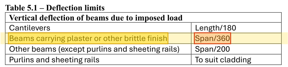
    For beams carrying plaster or other brittle finish, the imposed-load deflection limit is span/360.
    For beams carrying plaster or other brittle finish, the imposed-load deflection limit is span/360.Yellow: given parameter, row or columnOrange: value read from the table, boxed orange in the text too
Conclusion

Section strength and specified deflection Δ\Delta pass, but bending margin is smaller than B1's. Unrestrained B2 later gives a different LTB conclusion; there is no contradiction.

All the symbols of this example

SymbolsMeaning and Units
qq, ww, PPArea load kN/m², line load kN/m, point load kN
LL, RAR_A, RBR_BSpan in m or mm; end reactions in kN
MM, VVMoment demand in kNm; shear demand in kN
McM_c, VcV_c, MbM_bSection bending resistance in kNm, shear resistance in kN, LTB resistance in kNm
DD, dd, tt, TTOverall depth, classification web depth, web thickness and flange thickness; mm
AvA_v, II, SS, ZZShear area mm², second moment of area mm⁴, plastic/elastic moduli mm³
pyp_y, pbp_b, EEDesign yield/bending buckling strength and elastic modulus; N/mm²
Δ\Delta, η\etaDeflection mm; demand/resistance utilisation is dimensionless
GkG_k, QkQ_kUnfactored dead and imposed loads; kN/m or kN
hh, btribb_{trib}Slab thickness, tributary width; m

Video positions: 17 October 01:04:00 · 17 October 00:55:00 · 17 October 01:05:00 · 17 October 02:45:00

↑ Top