B1 floor beam: from slab load to strength and deflection (Complete Beam Walkthrough)
Task: Build line loads from the question, calculate design actions and interpret the lecturer's classification, shear, bending and deflection checks.
Go straight to Step 1 ↓Design flow for this type of question: Laterally restrained beam →
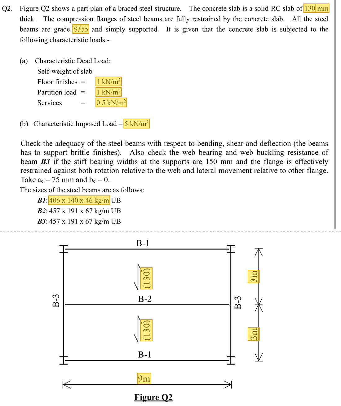
The question in short: A 9 m simply supported edge beam carries a 130 mm slab with beams 3 m apart, plus finishes, partitions, services and a 5 kN/m² imposed load. Decide whether a 406×140×46 UB in S355 is strong enough and does not bend too far.
| Given | Value and Unit |
|---|---|
| Geometry | Simply supported span 9 m; slab span (beam spacing) 3 m |
| Slab | Thickness 130 mm |
| Dead area loads | Floor finishes 1 kN/m²; partitions 1 kN/m²; services 0.5 kN/m² |
| Imposed area load | 5 kN/m² |
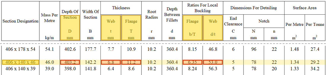
| Section | 406×140×46 UB (46 kg/m), S355; , , |
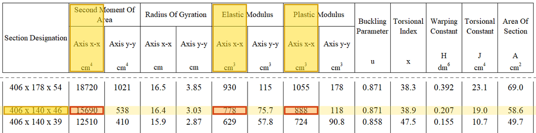
| Section properties | ; ; ; |
Yellow: values given in the question. The same values are marked where they are substituted in the steps below.
Orange box: values read directly from the Data File, the same values boxed orange in the lookup screenshots. A value interpolated between two table rows is a calculation, so it has no box.
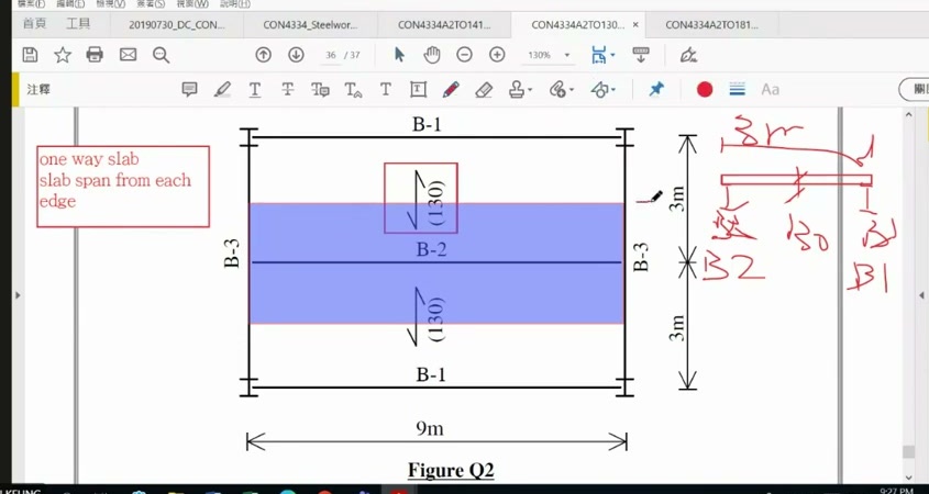
How to read this image: Locate edge beam B1, then use half the adjacent 3 m bay, 1.5 m, as tributary width for steps 1–3.
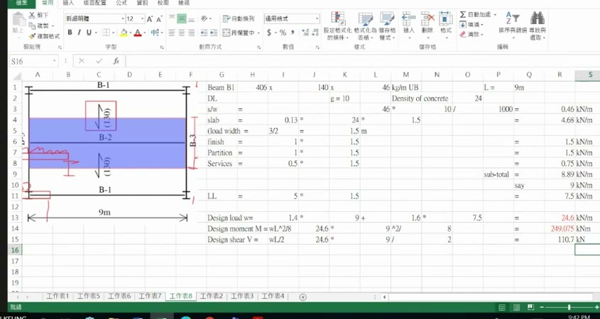
How to read this image: Read 0.46, 4.68, 1.5, 1.5 and 0.75 from top to bottom. Their sum corresponds to step 4 below.
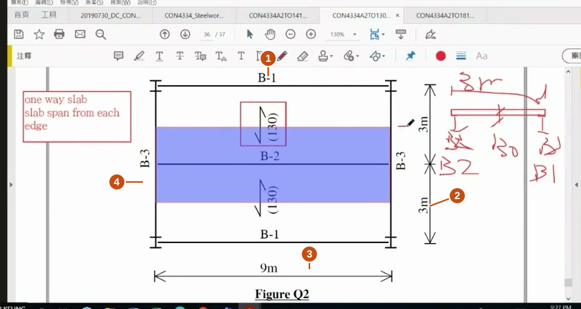
- ① B1 is the slab-edge beam. Identify the member to isolate first.
- ② The adjacent slab bay spans 3 m. The edge beam takes half, 1.5 m.
- ③ B1's own span is 9 m, used for reactions, moment and deflection.
- ④ B3 receives other beams' reactions. Do not copy B1's tributary width.
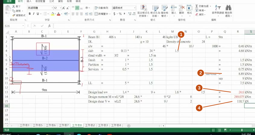
- ① Slab thickness 0.13 m × unit weight 24 × tributary width 1.5 gives 4.68 kN/m.
- ② Permanent line loads total 8.89; the lecturer adopts 9 for design.
- ③ Design line load 24.6 comes from .
- ④ The same load over 9 m gives and . Use a separate load for SLS.
Solution Route: Slab thickness→area load →line load →ULS actions→classification→shear/bending resistance →SLS deflection . The example begins on 3 October and continues on 17 October; sources are listed separately.
The area load on the slab goes first to the nearest beam. B1 is an edge beam with slab on one side only, so its tributary width is half the 3 m slab span.
- Area load on the slabTimes the 1.5 m tributary width
- Line load on B1ULS: 24.6 kN/m
- B1 in bending (midspan)Demand 249.075 kNmCapacity 315.24 kNmUtilisation 0.79
- B1 in shear (supports)Demand 110.7 kNCapacity 561.95 kNUtilisation 0.20
- Deflection (imposed load)Demand 19.92 mmCapacity 25 mmUtilisation 0.80 · closest to the limit
- Support reactions110.7 kN at each end, straight into the columns
- Step 1 · Identify tributary width
Why this step: The slab's weight is shared between the beams on each side. Fixing how wide a strip of slab this beam looks after is what later turns a floor load into a load on the beam.
The edge beam takes half the adjacent 3 m slab bay, giving 1.5 m. This follows slab spanning and support assumptions; it is not half the beam's 9 m span .
New symbols in this step- , : Slab thickness, tributary width; m
- Step 2 · Convert slab self-weight to area load
Why this step: The concrete slab is heavy and is a main part of the dead load. Finding its weight per square metre puts it in the same form as the other floor loads.
130 mm becomes 0.13 m, then it is multiplied by the unit weight of reinforced concrete, 24 kN/m³. The question does not give the unit weight; 24 kN/m³ is the usual value the lecturer uses.
Units: 130 mm divided by 1000 gives 0.13 m, because 1 m is 1000 mm; m times kN/m³ gives kN/m².
- Step 3 · Convert area load to line load
Why this step: Beam formulas work with load spread along the beam's length, so the weight of the slab strip is gathered into a line load sitting on the beam.
Multiplying by tributary width cancels one length dimension, leaving load per metre of beam.
Where the numbers come from: from Step 2.
- Step 4 · Add permanent loads individually
Why this step: Everything that stays on the beam for good is gathered into one figure, so the dead-load factor can be applied to it in one go later.
The beam self-weight of 46 kg/m is about 0.46 kN/m (the lecturer takes ); the three dead area loads are multiplied by the 1.5 m tributary width to become line loads . The lecturer rounds the total 8.89 to 9 for the rest of the design.
Where the numbers come from: from Step 3.
Units: kg/m times 10 gives N/m (1 kg weighs about 10 N); dividing by 1000 gives kN/m, because 1 kN is 1000 N.
- Step 5 · Imposed load and combination
Why this step: Load factors enlarge the loads to leave a safety margin. Imposed load is harder to predict than dead load, so it is enlarged more.
Multiply imposed area load by tributary width too, then combine using the lecturer's ULS factors.
New symbols in this step- , : Unfactored dead and imposed loads; kN/m or kN
- Step 6 · Draw the simply supported free body
Why this step: The supports must push up to hold all the load on the beam. This reaction is also the largest shear at the beam ends, which the shear check uses later.
Full-span UDL is symmetrical. Total design load 24.6×9=221.4 kN is shared equally between the supports.
New symbols in this step- , , : Span in m or mm; end reactions in kN
Where the numbers come from: from Step 5.
- Step 7 · Calculate maximum moment
Why this step: Moment measures how hard the load bends the beam, and it is greatest at midspan. This is the value the section must resist in bending.
Substitute midspan into , or use the derived simply supported UDL formula.
Where the numbers come from: from Step 5.
Load path · Load, shear force and bending momentThe beam takes the line load to its two ends: each reaction is half the total load. Shear is largest at the supports and zero at midspan; the moment is largest where the shear is zero. So shear is checked at the supports and bending at midspan. - Step 8 · Classify before using plastic resistance
Why this step: If the flange or web is too thin, it wrinkles locally before the section reaches its full strength. Classification confirms they are stocky enough to use for the capacity.
gives and . The lecturer's and both satisfy the corresponding Class 1 limits.
New symbols in this step- , , , : Overall depth, classification web depth, web thickness and flange thickness; mm
- , , : Design yield/bending buckling strength and elastic modulus; N/mm²
Data file lookup · Data Page 1 · Design strength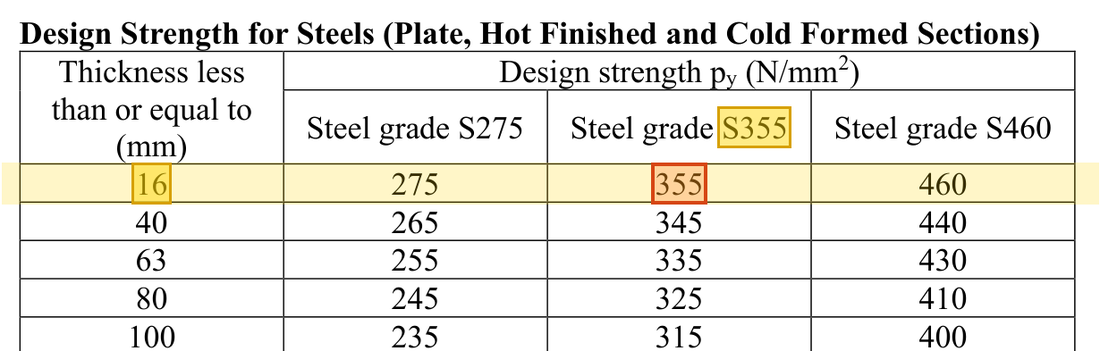
Flange thick: the row, S355 column gives . How the grade and thickness choose this row →Yellow: given parameter, row or columnOrange: value read from the table, boxed orange in the text too Data file lookup · Data Page 1 · Table 7.1 Limiting width-to-thickness ratios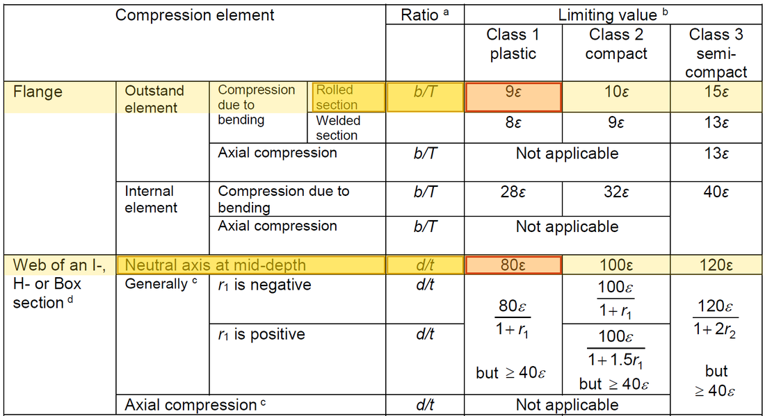
Rolled section: the Class 1 limits are 9ε for the outstand flange and 80ε for the web with the neutral axis at mid-depth. With , , so 9ε ≈ 7.92 and 80ε ≈ 70.4; and are both within the limits.Yellow: given parameter, row or columnOrange: value read from the table, boxed orange in the text too - Step 9 · Web shear area
Why this step: Shear is carried mainly by the upright web, so the area that resists it is found first, ready for the capacity in the next step.
For a rolled I-section, the course uses . Here is overall depth, not classification depth .
New symbols in this step- , , , : Shear area mm², second moment of area mm⁴, plastic/elastic moduli mm³
- Step 10 · Shear resistance and low-shear condition
Why this step: This guards against the web being sheared through near the supports. The capacity is the most shear the web can take before it yields.
Compare with , then separately decide whether unreduced bending resistance is available.
New symbols in this step- , , : Section bending resistance in kNm, shear resistance in kN, LTB resistance in kNm
Where the numbers come from: from Step 9.
Units: N/mm² times mm² gives N; dividing by 1000 gives kN, because 1 kN is 1000 N.
- Step 11 · Two different shear questions
Why this step: When shear is large it uses up part of the web's strength, leaving less for bending. With a low enough ratio, the moment capacity needs no reduction.
110.7<561.95 passes shear. Also, 110.7/561.95≈0.197<0.6 meets the course low-shear condition.
New symbols in this step- , : Moment demand in kNm; shear demand in kN
- Step 12 · Take the smaller bending resistance
Why this step: times is the bending strength when the whole section has yielded. The other candidate is an upper limit that stops the section starting to yield in everyday use.
Convert and from cm³ to mm³, then Nmm to kNm. Do not simply select the larger candidate.
Units: N/mm² times cm³, divided by 1000, gives kNm, because 1 cm³ is 1000 mm³ and 1 kNm is 1000000 Nmm.
- Step 13 · Bending comparison
Why this step: This guards against the midspan section yielding in bending. A ratio below one means the moment from the loads is within what the section can resist.
249.075<315.24 passes cross-sectional bending. This does not automatically establish freedom from LTB.
- Step 14 · Start a separate SLS data row
Why this step: Deflection is about everyday use, not collapse, so the load that really occurs is used, without load factors.
The lecturer uses unfactored imposed load 7.5 kN/m=7.5 N/mm for deflection , not 24.6. Use and .
- Step 15 · Choose the correct deflection model and substitute
Why this step: This finds how far the beam sags at midspan. Too much sag makes the floor feel unsafe and can crack finishes and partitions.
This is a simply supported full-span UDL, so use 5wL⁴/(384EI) with course .
New symbols in this step- , : Deflection mm; demand/resistance utilisation is dimensionless
Where the numbers come from: from Step 5.
Units: in cm⁴ times 10^4 gives mm⁴, because 1 cm is 10 mm, multiplied four times. 7.5 kN/m equals 7.5 N/mm, and 9 m is written as 9000 mm.
Data file lookup · Data Page 1 · Steel properties
Data Page 1, steel properties: modulus of elasticity (printed as 205,000).Yellow: given parameter, row or columnOrange: value read from the table, boxed orange in the text too - Step 16 · Compare with this problem's limit
Why this step: The limit grows with the span. An actual deflection below the limit means the beam does not bend too far in everyday use.
The applicable limit is . Convert it to the same mm units before comparison.
Units: The 9 m span times 1000 gives 9000 mm, because 1 m is 1000 mm, so the limit and the deflection are both in mm.
Data file lookup · Data Page 2 · Table 5.1 Deflection limits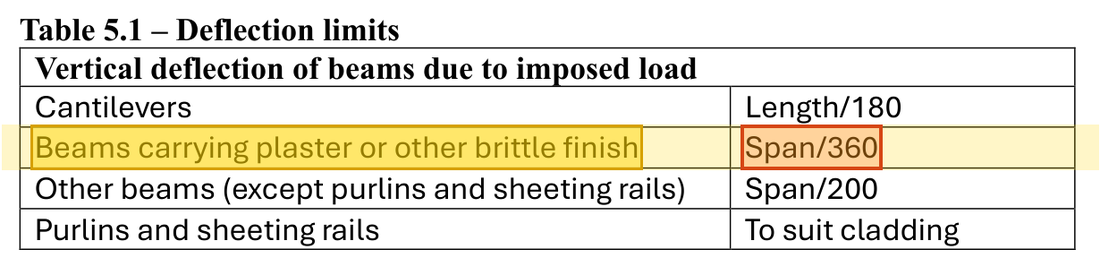
For beams carrying plaster or other brittle finish, the imposed-load deflection limit is span/360.Yellow: given parameter, row or columnOrange: value read from the table, boxed orange in the text too
The classification, shear, low-shear bending and specified SLS deflection checks all pass. A complete member design still needs LTB, local web bearing and other checks for the actual lateral restraints and supports; these results do not cover every check.
All the symbols of this example
| Symbols | Meaning and Units |
|---|---|
| , , | Area load kN/m², line load kN/m, point load kN |
| , , | Span in m or mm; end reactions in kN |
| , | Moment demand in kNm; shear demand in kN |
| , , | Section bending resistance in kNm, shear resistance in kN, LTB resistance in kNm |
| , , , | Overall depth, classification web depth, web thickness and flange thickness; mm |
| , , , | Shear area mm², second moment of area mm⁴, plastic/elastic moduli mm³ |
| , , | Design yield/bending buckling strength and elastic modulus; N/mm² |
| , | Deflection mm; demand/resistance utilisation is dimensionless |
| , | Unfactored dead and imposed loads; kN/m or kN |
| , | Slab thickness, tributary width; m |
Video positions: 3 October Recording B 02:25:00 · 3 October Recording B 02:40:00 · 3 October Recording B 02:50:00 · 17 October 00:25:00 · 17 October 00:26:20