Companion slides and quick-reference notes
Open “Animation lab” beside a teaching step for a visual explanation or a walkthrough of its original expressions. Models are illustrative; source answers remain unchanged.
These are teaching notes for every slide in the four companion presentations. Each original slide remains readable locally. The linked chapter supplies the full derivation and worked applications; corrections to compressed slide statements are explicit.
PPT/Structural Steelwork Design L1.pptx · slide 1: Introduction: what you are learning
A design answer compares a demand caused by loads with a resistance supplied by steel. First calculate the loads and forces; then check the chosen component. A failure of any required check means the proposal needs revision.
Study the full explanation and applications.
Animation labFollow the calculation sequence
Supplement to the original lesson. Enable JavaScript to play, step through calculations and rotate 3D models. The following explanation remains readable offline.
- Locate the load, supports, connection geometry and any stated assumptions.
- Keep given values, table lookups and calculated values distinct; reconcile their units.
- The calculation player steps through the existing expressions in their original order.
- Compare demand with resistance or the relevant limit. Keep missing inputs and conditional conclusions explicit.
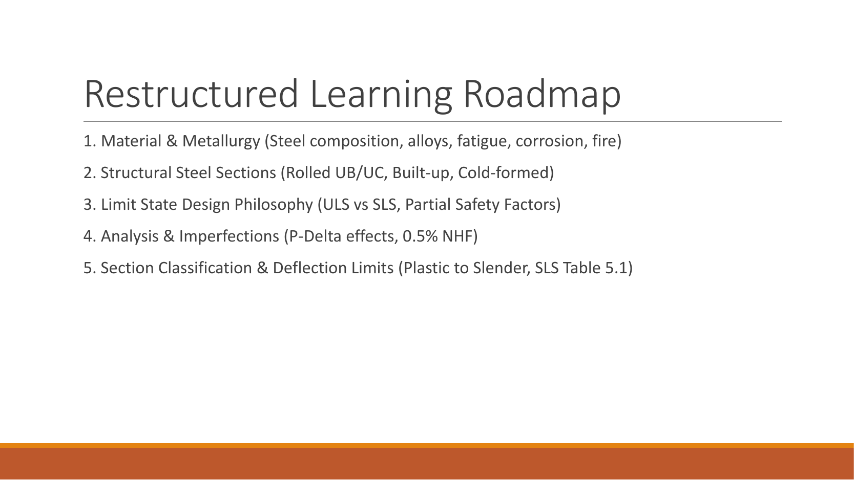
PPT/Structural Steelwork Design L1.pptx · slide 2: The course roadmap
Learn foundations before connections, beams and columns. The same equilibrium equations recur: vertical forces balance, horizontal forces balance, and moments balance. The shape and restraints decide which resistance checks are needed.
Study the full explanation and applications.
Animation labFollow the calculation sequence
Supplement to the original lesson. Enable JavaScript to play, step through calculations and rotate 3D models. The following explanation remains readable offline.
- Locate the load, supports, connection geometry and any stated assumptions.
- Keep given values, table lookups and calculated values distinct; reconcile their units.
- The calculation player steps through the existing expressions in their original order.
- Compare demand with resistance or the relevant limit. Keep missing inputs and conditional conclusions explicit.
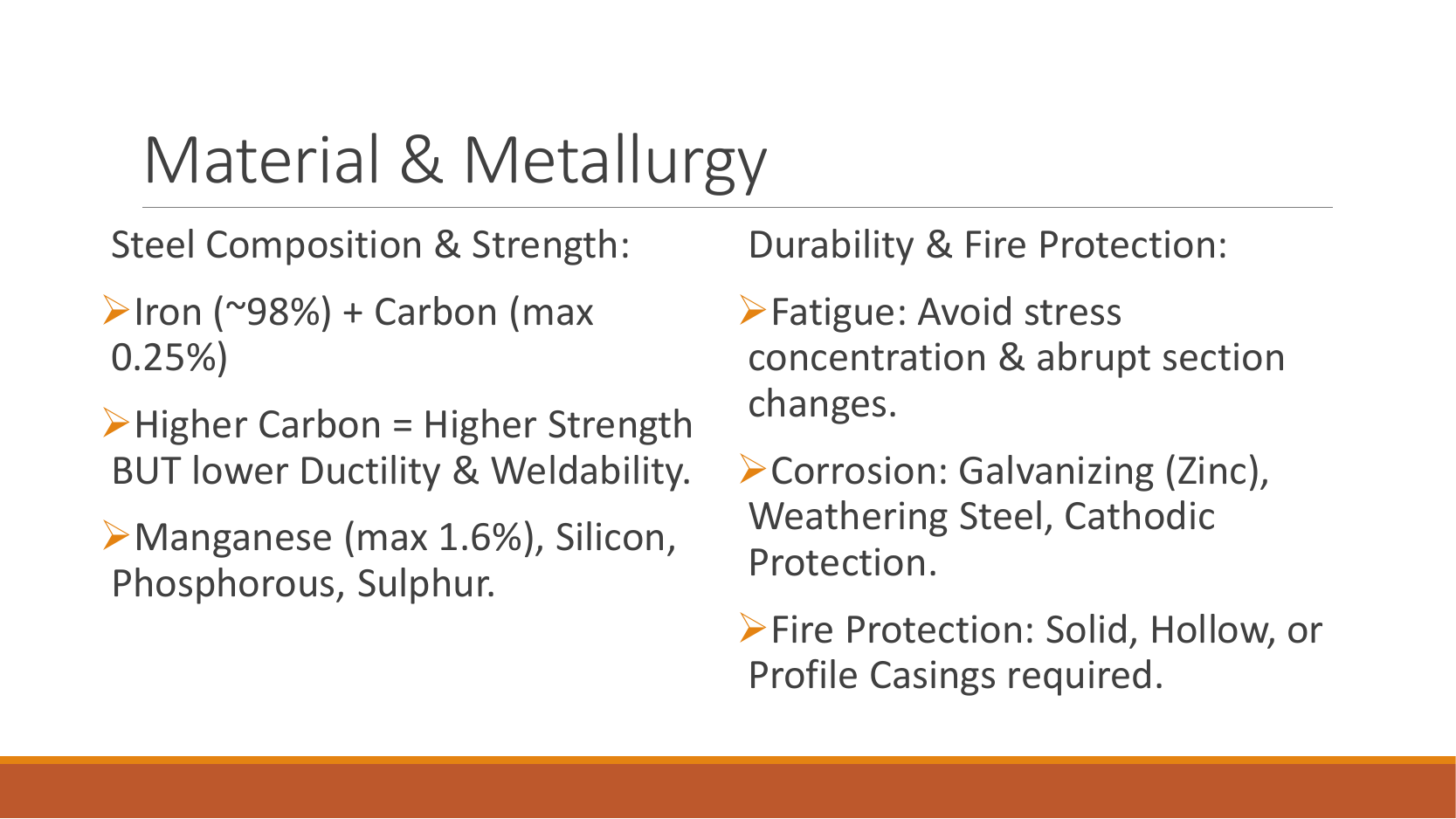
PPT/Structural Steelwork Design L1.pptx · slide 3: Steel behaviour and protection
The slide describes steel as mostly iron, with controlled carbon and manganese. Carbon raises strength but can reduce ductility and weldability. Fatigue is repeated-load crack growth; corrosion removes material; heat reduces stiffness and strength. For an exam explanation, link each protection method to the damage mechanism it prevents.
Study the full explanation and applications.
Animation labElasticity, yielding and ductility
Supplement to the original lesson. Enable JavaScript to play, step through calculations and rotate 3D models. The following explanation remains readable offline.
- Stress is force divided by area. Strain measures change in length relative to original length.
- Before yielding, stress is approximately . E controls the elastic slope.
- Further strain includes permanent deformation. Higher yield strength does not by itself increase E.
- Strength, stiffness and ductility answer different questions. This schematic is not a measured stress–strain curve.
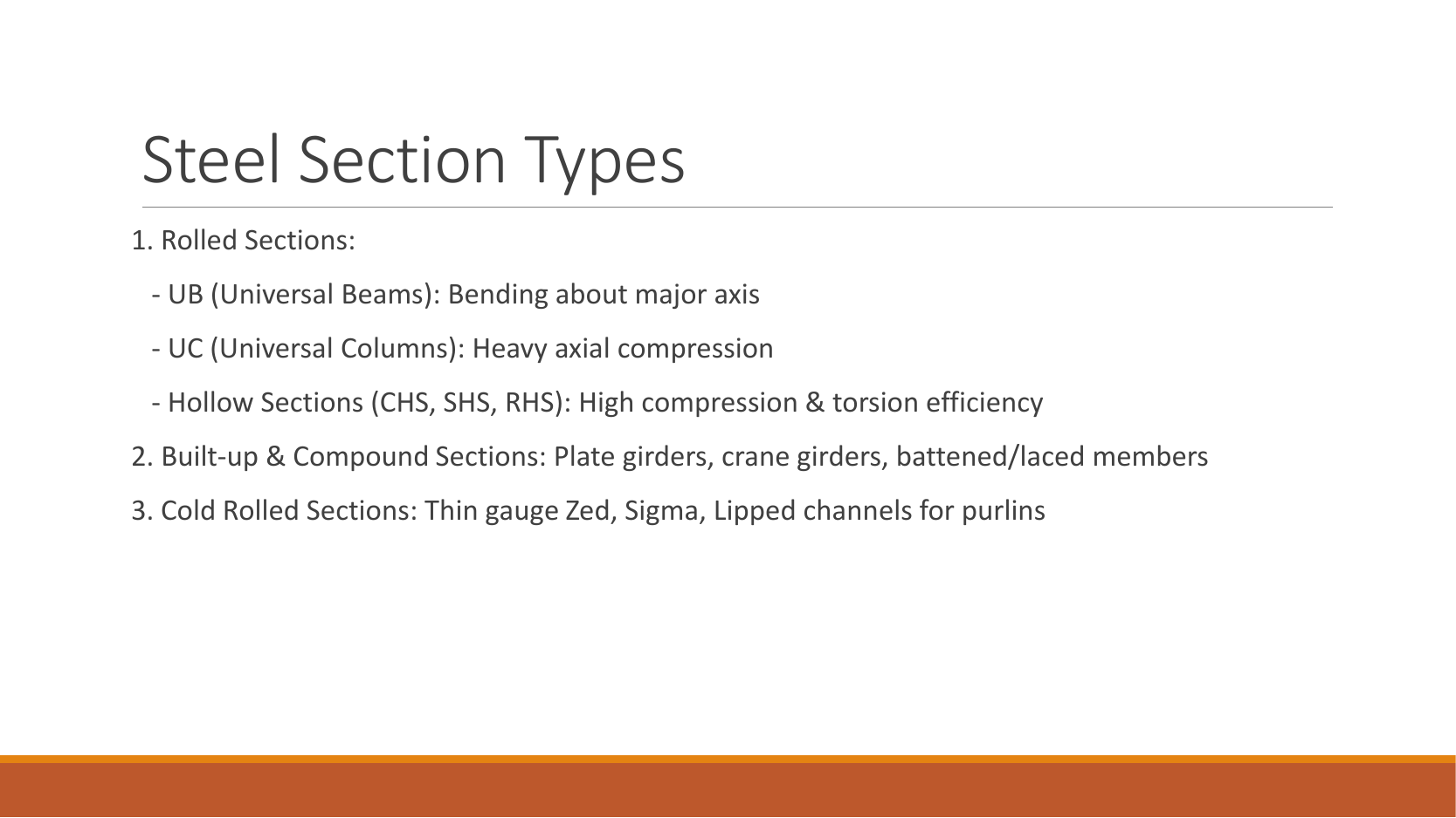
PPT/Structural Steelwork Design L1.pptx · slide 4: Recognise the section
An I or H section has two flanges and a web; angles and channels are open, unsymmetrical shapes. Rolled means formed hot at a mill. Built-up means plates or sections joined into a member. Identify the section family before choosing dimensions, axes or buckling curves.
Study the full explanation and applications.
Animation labExplore section geometry and axes
Supplement to the original lesson. Enable JavaScript to play, step through calculations and rotate 3D models. The following explanation remains readable offline.
- The flanges are the wide plates; the web connects them. Rotate the I-section to see both.
- The same section has different stiffness and resistance about its two principal axes.
- I controls elastic curvature; is elastic section modulus. Plastic modulus S comes from plastic stress blocks.
- Nominal section labels are not every actual dimension. Keep the row, axis and units together.
PPT/Structural Steelwork Design L1.pptx · slide 5: ULS versus SLS
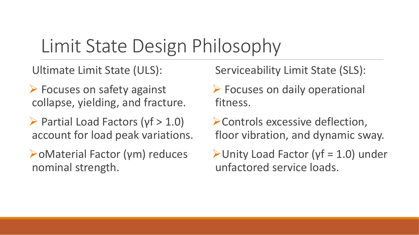
ULS checks strength and stability using the prescribed factored load combination. SLS checks usable behaviour such as deflection. Do not carry the ULS load into an imposed-load-only deflection check. is permanent load, imposed load and wind action.
Study the full explanation and applications.
Animation labTwo different design questions
Supplement to the original lesson. Enable JavaScript to play, step through calculations and rotate 3D models. The following explanation remains readable offline.
- ULS compares factored actions with the applicable resistance to yielding, rupture or instability.
- SLS checks movement, vibration or another specified use requirement.
- A beam can be strong enough but deflect too much. The two checks need their own loads and denominators.
- A resistance pass cannot stand in for a serviceability pass. Complete all requested checks.
PPT/Structural Steelwork Design L1.pptx · slide 6: Choose a load combination
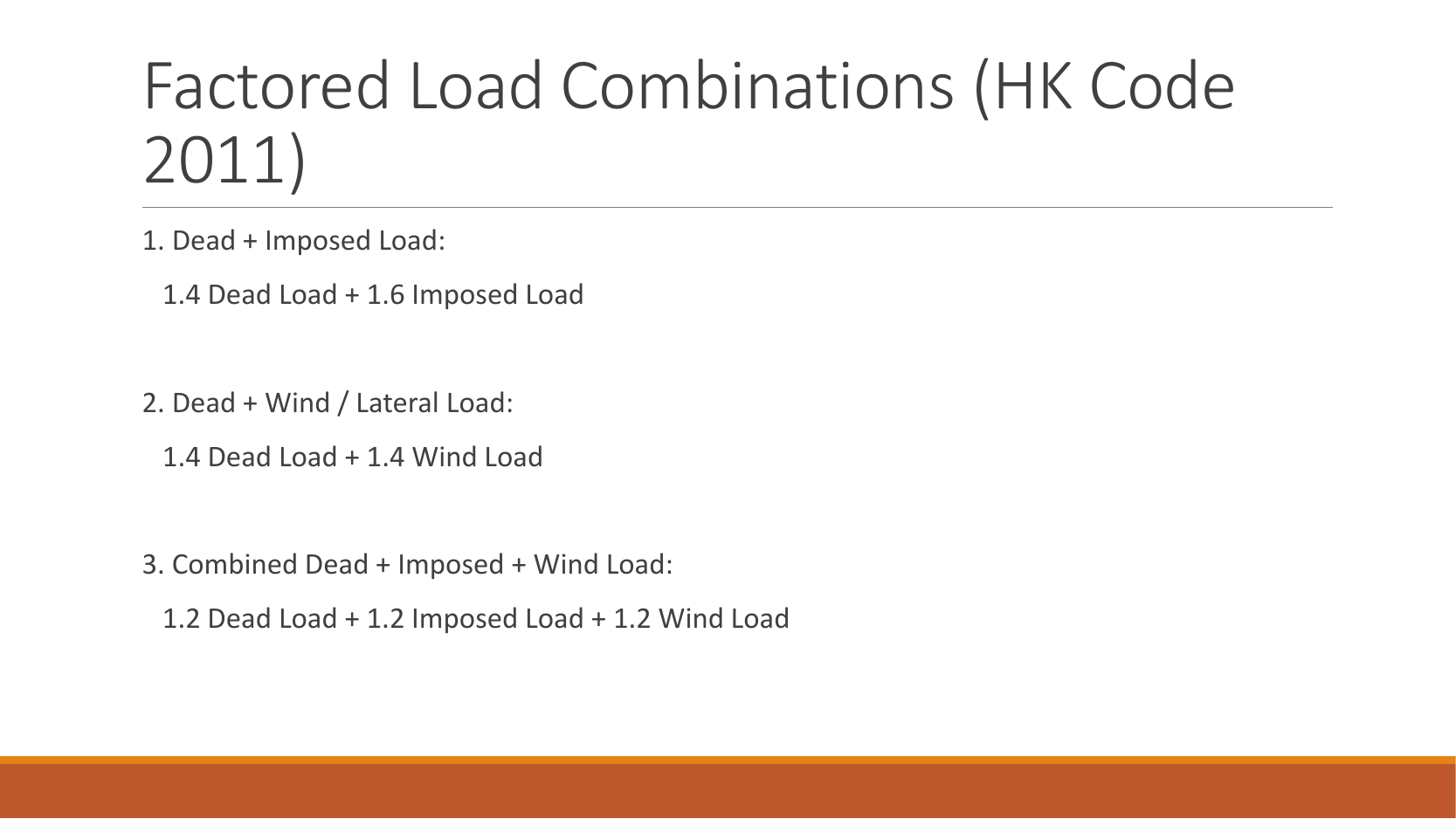
The slide lists , and . These are different cases, not extra multipliers applied one after another. Choose the relevant adverse combination and consider whether an action is beneficial. For example, and gives .
Study the full explanation and applications.
Animation labFrom characteristic to design load
Supplement to the original lesson. Enable JavaScript to play, step through calculations and rotate 3D models. The following explanation remains readable offline.
- G is permanent load; Q is imposed load. A surface load and a line load also have different units.
- This illustration uses the course gravity case . Other combinations in the original text retain their own factors.
- For illustrative , change Q and watch each separate contribution.
- Do not carry this ULS total automatically into deflection. Follow the stated SLS load case.
PPT/Structural Steelwork Design L1.pptx · slide 7: Choose the analysis model
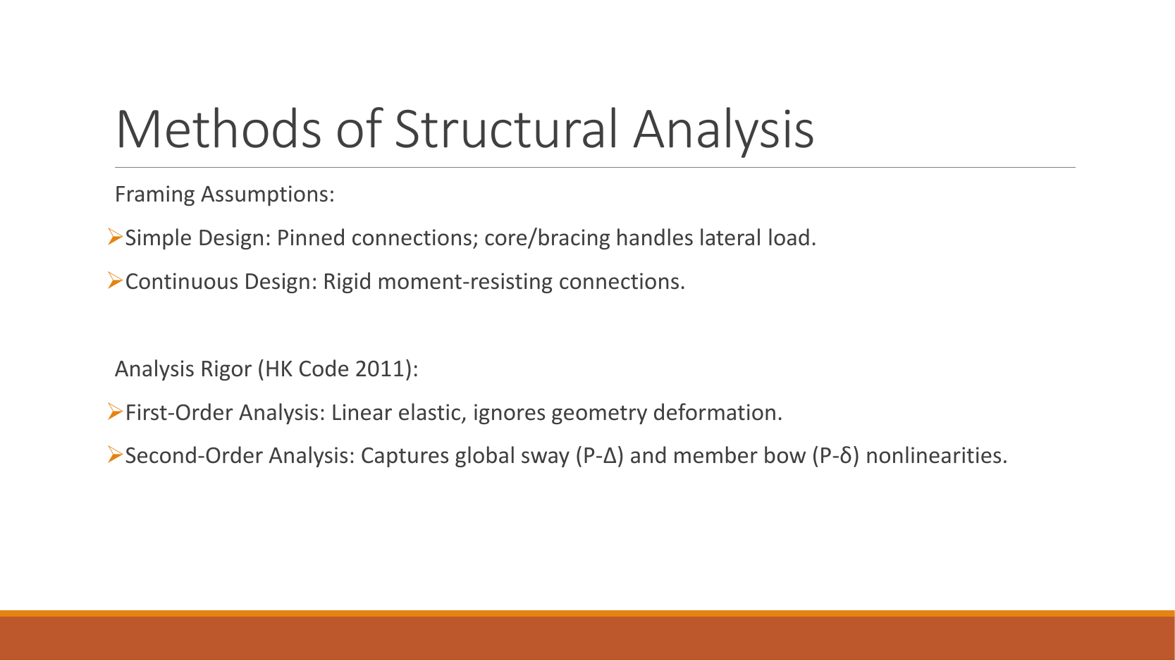
Simple construction treats joints as nominally pinned for global analysis; continuous construction transfers joint moments. First-order analysis uses the undeformed shape; second-order analysis includes extra moments caused by displacement under axial force. Do not infer moment fixity from a visually thick line in a sketch.
Study the full explanation and applications.
Animation labRestraints, sway and imperfections
Supplement to the original lesson. Enable JavaScript to play, step through calculations and rotate 3D models. The following explanation remains readable offline.
- A frame needs a defined path for horizontal force as well as gravity.
- Pinned joints alone do not provide frame moment resistance; sway restraint needs a real structural system.
- Diagonal bracing carries horizontal action through axial forces. This sketch does not assign a numerical frame classification.
- Use the specified imperfection/notional-force model and critical-load criteria. Avoid counting alternative imperfection models twice.
PPT/Structural Steelwork Design L1.pptx · slide 8: Imperfections and notional forces
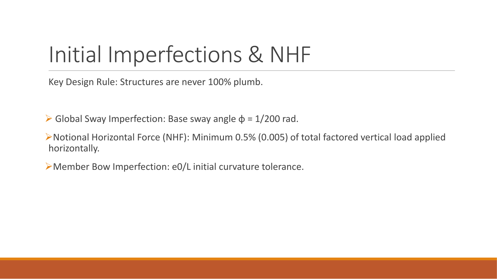
Real members are not perfectly straight or vertical. The slide uses a nominal frame imperfection and notional horizontal force times vertical load. For a vertical action, that force is . Apply it in the stated analysis case; it does not replace actual wind automatically. Member initial bow and frame lean are different imperfections.
Study the full explanation and applications.
Animation labRestraints, sway and imperfections
Supplement to the original lesson. Enable JavaScript to play, step through calculations and rotate 3D models. The following explanation remains readable offline.
- A frame needs a defined path for horizontal force as well as gravity.
- Pinned joints alone do not provide frame moment resistance; sway restraint needs a real structural system.
- Diagonal bracing carries horizontal action through axial forces. This sketch does not assign a numerical frame classification.
- Use the specified imperfection/notional-force model and critical-load criteria. Avoid counting alternative imperfection models twice.
PPT/Structural Steelwork Design L1.pptx · slide 9: Serviceability limits
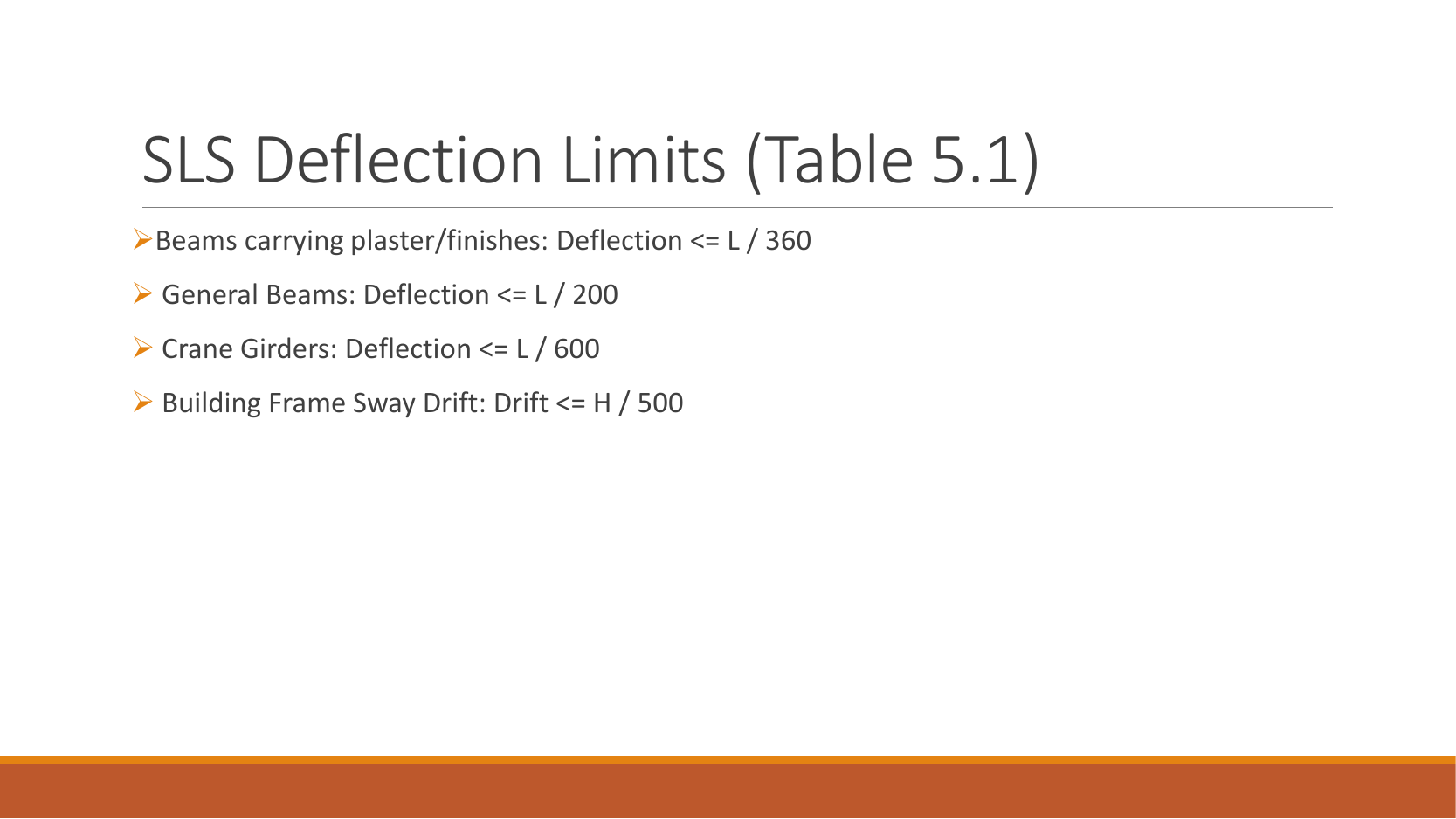
For imposed-load vertical deflection, use the applicable row: brittle finishes , other beams , cantilevers . The slide also mentions crane and frame ; the full course table states the conditions, so a limit must be selected by function and displacement type. A span of at permits .
Study the full explanation and applications.
Animation labSee stiffness and deflection
Supplement to the original lesson. Enable JavaScript to play, step through calculations and rotate 3D models. The following explanation remains readable offline.
- Use the specified SLS load, span and support arrangement. The demonstrator has a full-span UDL.
- The loaded beam bends; the deformation is exaggerated so its shape can be seen.
- For a simply supported full-span UDL, . Double L with w, E and I unchanged: δ becomes 16 times as large.
- The readout uses , and . Select the finish/support-specific limit from the original table.
PPT/Structural Steelwork Design L1.pptx · slide 10: Strength depends on thickness
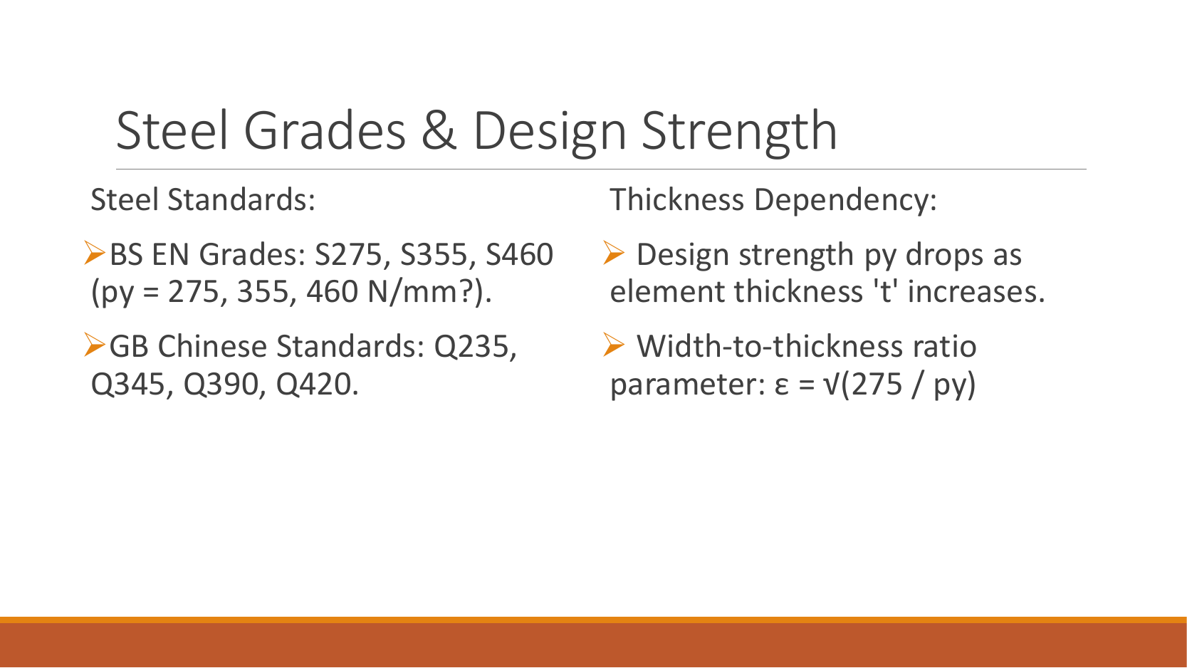
S355 is a grade name, not a promise that every thickness has design strength . Read the maximum-thickness row: a flange falls in the row, giving . Then . Use the controlling plate thickness for the relevant property check.
Study the full explanation and applications.
Animation labRead a table without losing the keys
Supplement to the original lesson. Enable JavaScript to play, step through calculations and rotate 3D models. The following explanation remains readable offline.
- Name the required property: material strength, section property, buckling strength or a moment factor.
- Keep section size, steel grade, thickness band, curve and axis as separate lookup keys.
- , and require different conversion powers. Do not use adjacent columns interchangeably.
- Use bracketing rows within the same valid column. The original page remains the source of all table values.
PPT/Structural Steelwork Design L1.pptx · slide 11: Section classes
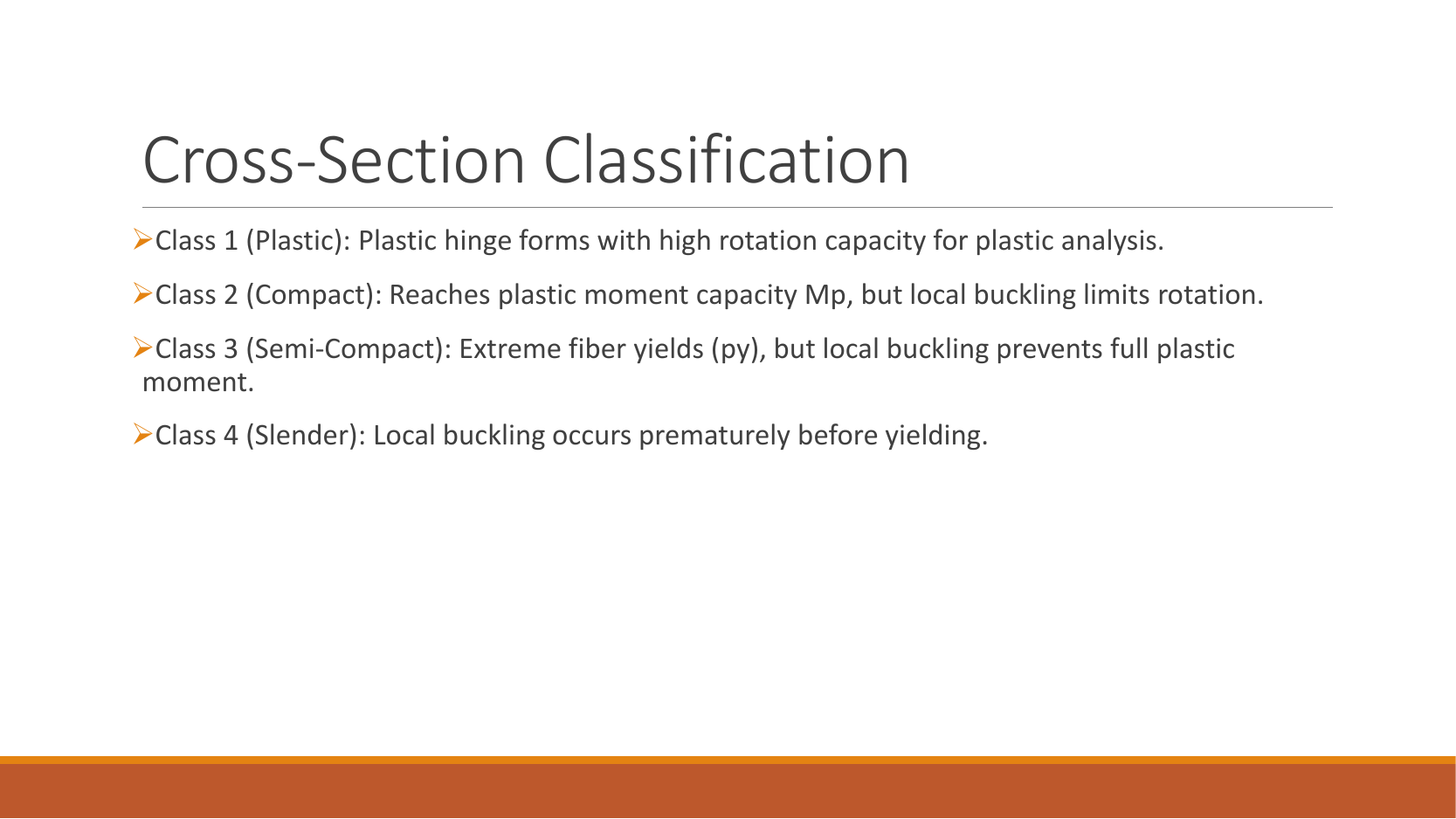
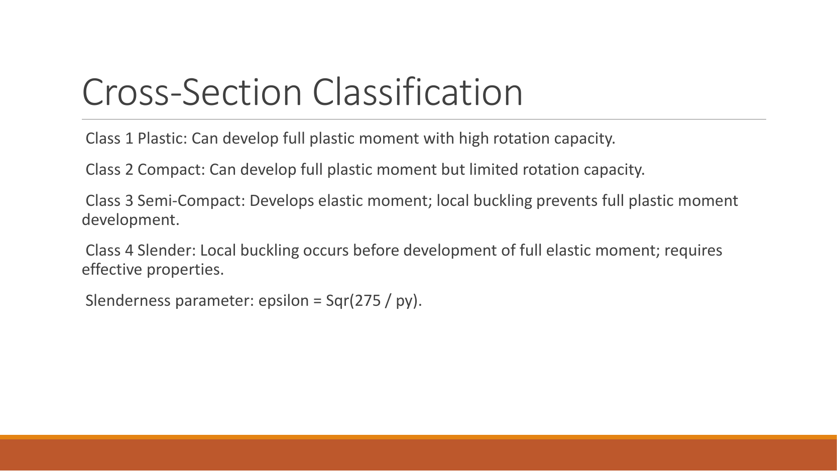
Class 1 permits a plastic hinge with rotation; Class 2 reaches plastic moment with less rotation; Class 3 uses elastic capacity; Class 4 requires effective properties. Check flange and web separately under their actual stress distributions, then take the worse class. A stocky flange does not make a slender web Class 1.
Study the full explanation and applications.
Animation labWhy thin elements buckle locally
Supplement to the original lesson. Enable JavaScript to play, step through calculations and rotate 3D models. The following explanation remains readable offline.
- The flange outstand and web have different widths, thicknesses and edge support conditions.
- A thinner plate can wrinkle locally before the complete member loses stability.
- Class 1 allows plastic rotation; Class 2 reaches plastic resistance; Class 3 reaches elastic resistance; Class 4 requires effective properties.
- Check every relevant compression element with the supplied limits and stress distribution. The deformation shown is qualitative.
PPT/Structural Steelwork Design L1.pptx · slide 12: Turn discussion into a self-test
Without notes, explain why a beam can pass bending yet fail LTB, why a column has two slenderness ratios, and why bolt diameter differs from hole diameter. Answers: instability depends on unrestrained length; radii/restraints differ by axis; holes need clearance. Return to the linked chapters if you cannot explain the mechanism.
Study the full explanation and applications.
Animation labA beam bends sideways and twists
Supplement to the original lesson. Enable JavaScript to play, step through calculations and rotate 3D models. The following explanation remains readable offline.
- For the illustrated sagging beam the top flange is compressed.
- The unrestrained compression flange can move sideways while the complete cross-section twists.
- Only effective restraints divide the member into unbraced segments. They do not automatically add vertical supports.
- Use the segment effective length, section properties and matching moment factor. This is an exaggerated mode shape, not a calculated displacement.
PPT/Joint Connections L2.pptx · slide 1: Joint connections: purpose
A connection transfers forces between members. Sketch the complete force path before calculating an individual bolt or weld; a strong fastener cannot rescue a weak connected plate.
Study the full explanation and applications.
Animation labCount the bolt shear planes
Supplement to the original lesson. Enable JavaScript to play, step through calculations and rotate 3D models. The following explanation remains readable offline.
- Load must cross an interface between the connected plates.
- A lap joint gives one shear plane through a bolt.
- A symmetric double-cover joint may provide two shear planes. Count load-transfer interfaces, not just visible plates.
- Use the source’s area and shear strength. Then check bearing, plate resistance and detailing separately.
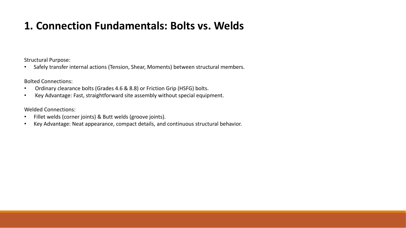
PPT/Joint Connections L2.pptx · slide 2: Bolts and welds
Bolts transfer force through shear, bearing, tension, or specified friction-grip action. Welds transfer force through fused metal along an effective throat. This course’s ordinary-bolt equations do not establish slip resistance for a friction-grip joint.
Study the full explanation and applications.
Animation labCount the bolt shear planes
Supplement to the original lesson. Enable JavaScript to play, step through calculations and rotate 3D models. The following explanation remains readable offline.
- Load must cross an interface between the connected plates.
- A lap joint gives one shear plane through a bolt.
- A symmetric double-cover joint may provide two shear planes. Count load-transfer interfaces, not just visible plates.
- Use the source’s area and shear strength. Then check bearing, plate resistance and detailing separately.
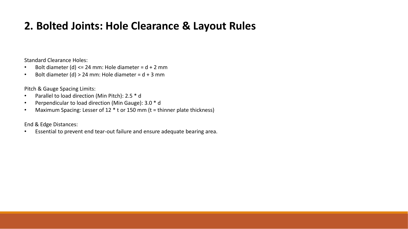
PPT/Joint Connections L2.pptx · slide 3: Read the bolt layout
Pitch runs along the force transfer direction; gauge separates lines; end distance is from a hole centre to the end in that direction. Hole diameter is used in net area, nominal bolt diameter in projected bearing. Check standard-hole clearance and minimum/maximum spacing before claiming a layout is valid.
Study the full explanation and applications.
Animation labBolt centres, holes and edges
Supplement to the original lesson. Enable JavaScript to play, step through calculations and rotate 3D models. The following explanation remains readable offline.
- Hole diameter d₀ differs from nominal bolt diameter d. Net-section deductions use the specified hole.
- Pitch runs along the load direction; gauge measures spacing across rows.
- End and edge distances start at the hole centre. The remaining ligament starts at the hole boundary.
- Minimum spacing, edge distances, grip and plate thickness come from the specified rules, not this scaled illustration.
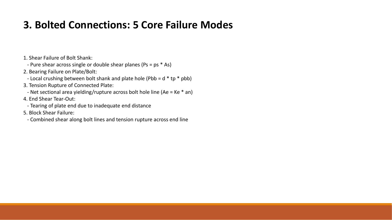
PPT/Joint Connections L2.pptx · slide 4: Five failure modes
Inspect bolt shear, bolt tension where present, bearing of the bolt/connected part, tensile rupture of the net section and block shear. For each mode draw what separates or deforms. Capacity is the smallest applicable resistance along the force path, not the sum of unrelated failure resistances.
Study the full explanation and applications.
Animation labSeparate the block-shear paths
Supplement to the original lesson. Enable JavaScript to play, step through calculations and rotate 3D models. The following explanation remains readable offline.
- A block containing the connection can detach from the surrounding plate.
- The paths parallel to the applied force carry shear.
- The closing path across the end of the block carries tension.
- Use the specified gross/net deductions and resistance expression. This is different from a single straight net-section fracture.
PPT/Joint Connections L2.pptx · slide 5: Weld types and inspection
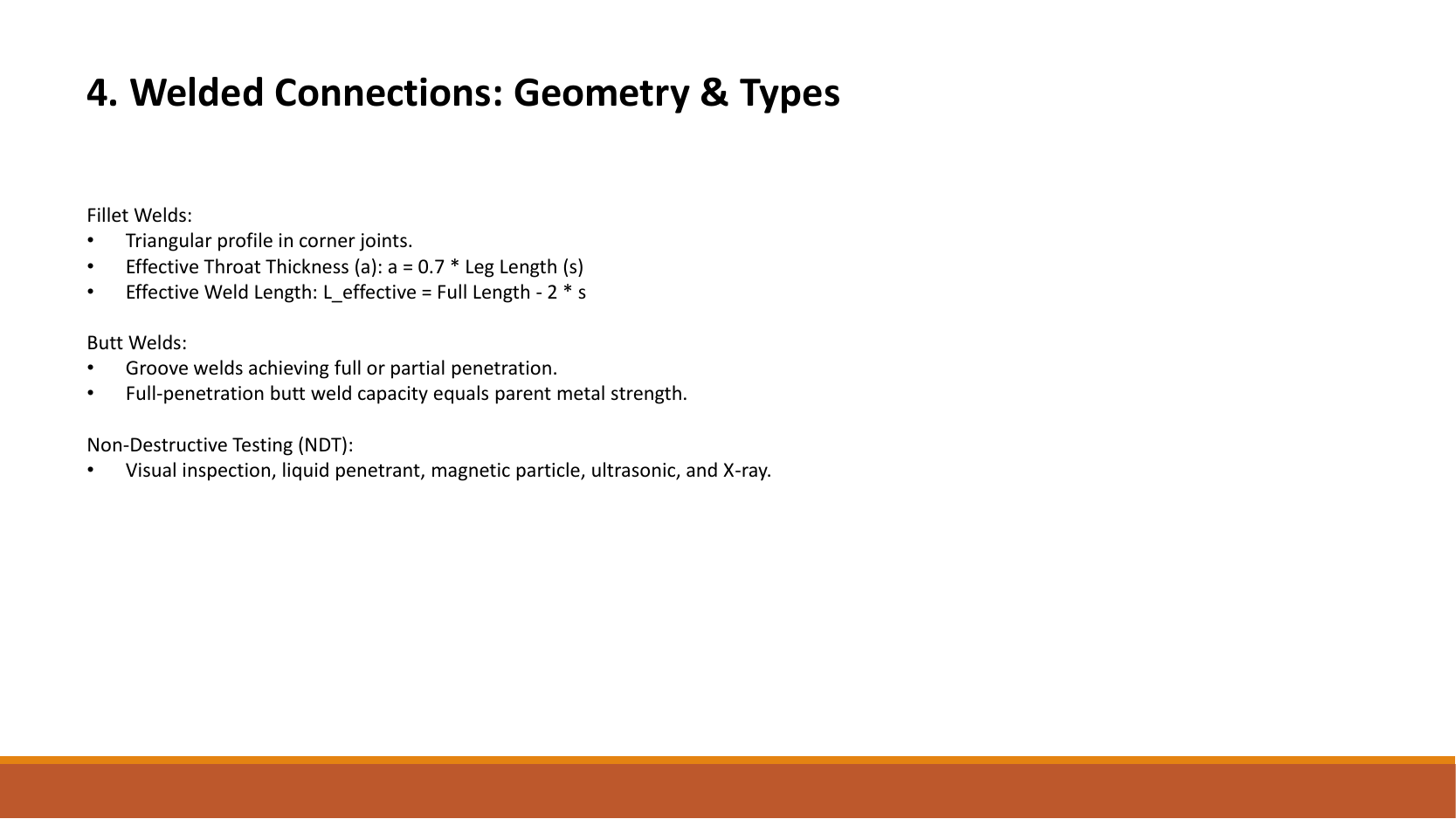
A fillet weld joins surfaces at an angle and is sized by leg length. A butt weld joins prepared edges; penetration matters. Visual inspection checks shape and visible defects; penetrant and magnetic-particle methods seek surface defects; ultrasonic and radiographic methods seek internal defects. Strong arithmetic assumes acceptable fabrication.
Study the full explanation and applications.
Animation labFrom fillet leg to effective throat
Supplement to the original lesson. Enable JavaScript to play, step through calculations and rotate 3D models. The following explanation remains readable offline.
- An equal-leg fillet between perpendicular plates has an approximately right-triangular section.
- For this geometry, throat . It is shorter than the leg.
- Effective resisting area = . With here, capacity per length is .
- Use the course end allowances, minimum size and length rules; increasing the geometric length alone does not resolve every detailing check.
PPT/Joint Connections L2.pptx · slide 6: The unnumbered 6 mm weld calculation
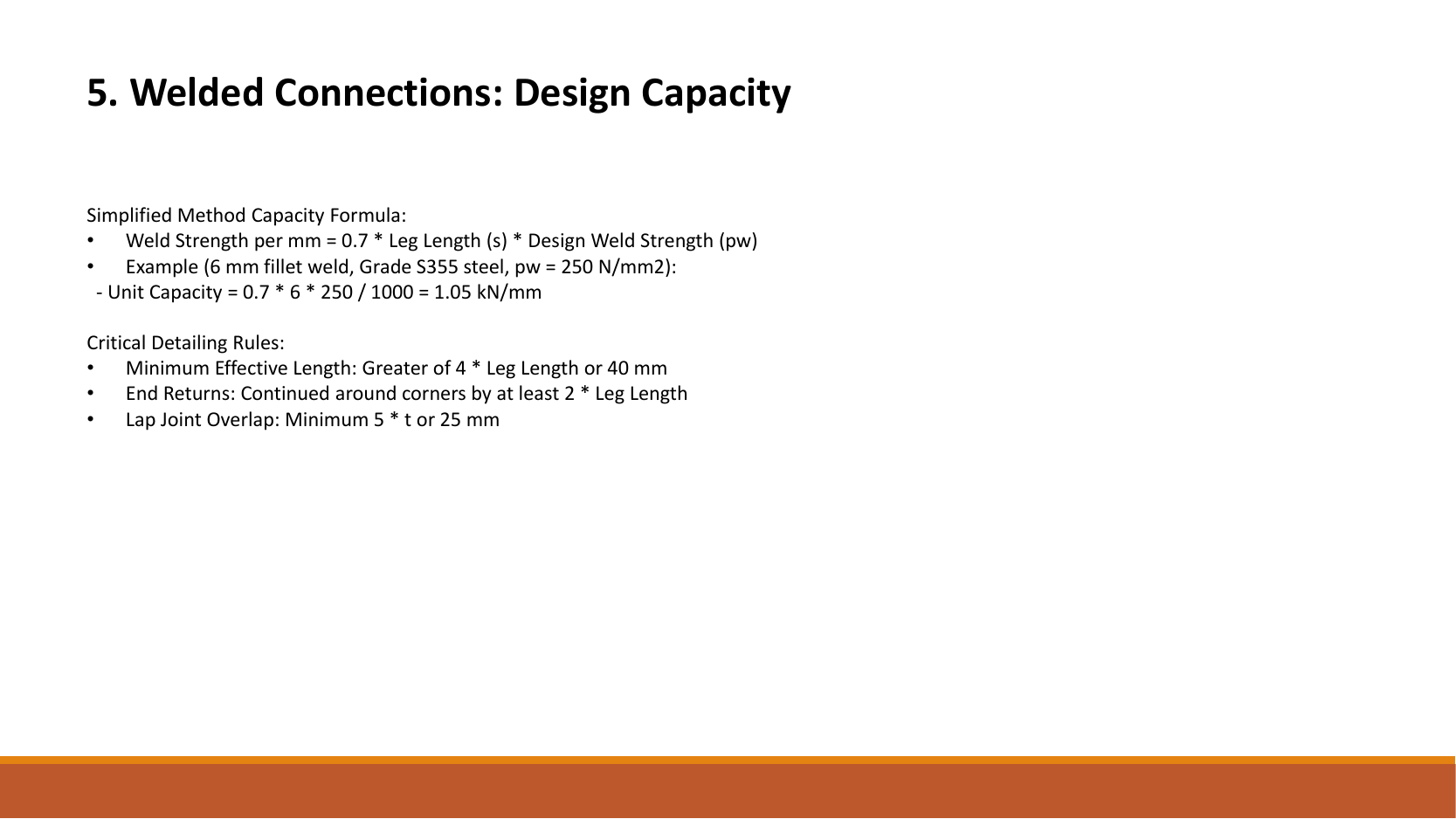
Given S355 steel and Class 42 electrode, Table 9.2a gives . A fillet of leg has throat . Per millimetre of effective weld, area=; resistance=. Thus . Required length for direct force is effective; physical straight length is before other detailing constraints.
Study the full explanation and applications.
Animation labFrom fillet leg to effective throat
Supplement to the original lesson. Enable JavaScript to play, step through calculations and rotate 3D models. The following explanation remains readable offline.
- An equal-leg fillet between perpendicular plates has an approximately right-triangular section.
- For this geometry, throat . It is shorter than the leg.
- Effective resisting area = . With here, capacity per length is .
- Use the course end allowances, minimum size and length rules; increasing the geometric length alone does not resolve every detailing check.
PPT/Joint Connections L2.pptx · slide 7: Recognise eccentricity in three dimensions
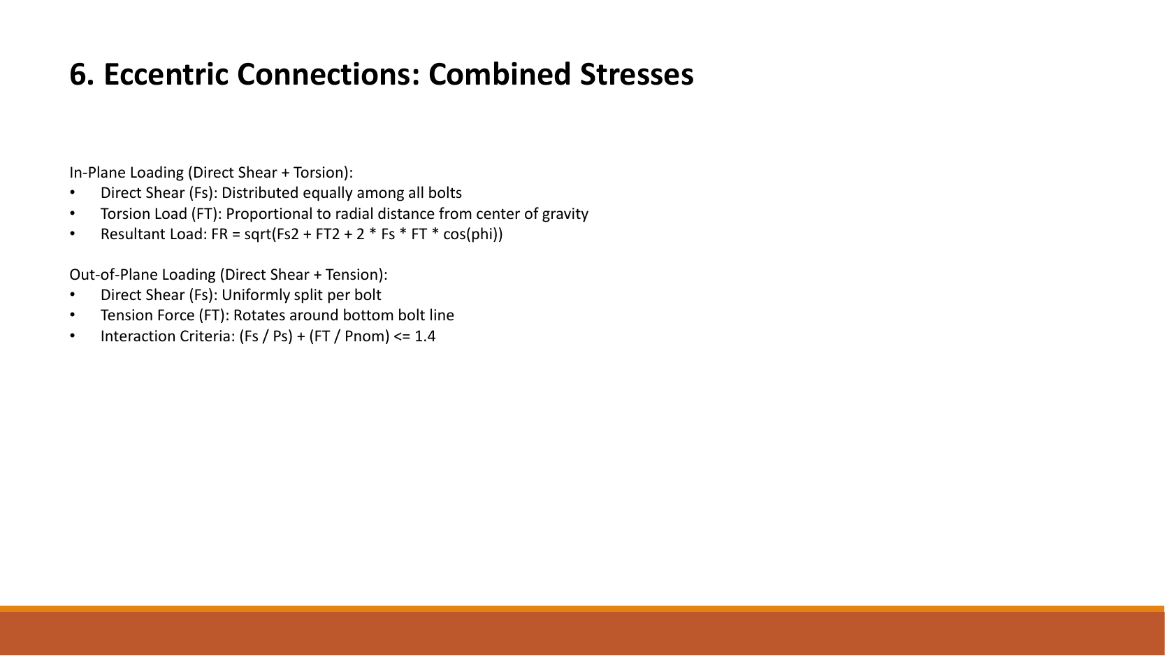
An in-plane force rotates the bolt/weld group about its centroid and gives direct plus torsional shear. An out-of-plane bracket load opens the joint and creates fastener tension. For bolts, check individual shear and tension and ; . The interaction limit is , not .
Study the full explanation and applications.
Animation labAdd direct and torsional bolt forces
Supplement to the original lesson. Enable JavaScript to play, step through calculations and rotate 3D models. The following explanation remains readable offline.
- Assign signed coordinates to the bolts relative to the group centroid.
- For the equal-bolt elastic model, the direct force is per bolt.
- Moment magnitude is ; its sign follows the load direction. For signed M: , , .
- Add signed x and y components at each bolt, then take the resultant. The longest arrow shows the critical bolt in this illustration.
PPT/Joint Connections L2.pptx · slide 8: A reusable connection workflow
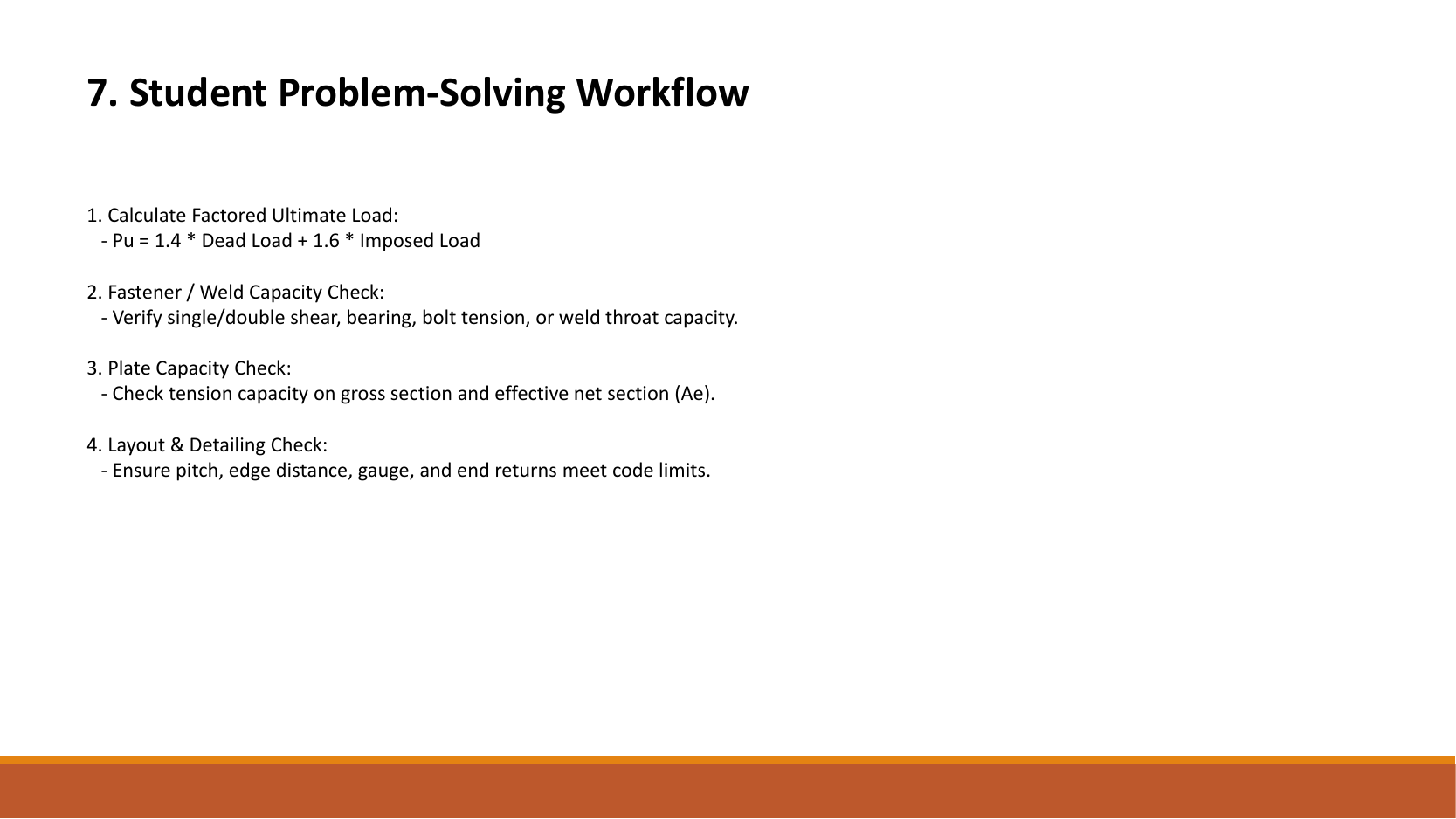
Resolve factored actions; classify force direction; label geometry; calculate individual fastener demand; calculate all applicable fastener and plate resistances; check layout; state the governing result and assumptions. See the worked example before attempting the corresponding tutorial with the answer hidden.
Study the full explanation and applications.
Animation labFollow the calculation sequence
Supplement to the original lesson. Enable JavaScript to play, step through calculations and rotate 3D models. The following explanation remains readable offline.
- Locate the load, supports, connection geometry and any stated assumptions.
- Keep given values, table lookups and calculated values distinct; reconcile their units.
- The calculation player steps through the existing expressions in their original order.
- Compare demand with resistance or the relevant limit. Keep missing inputs and conditional conclusions explicit.
PPT/Steel Beam Design L3.pptx · slide 1: Beam design
A beam mainly resists transverse load by bending and shear. Its vertical supports and sideways restraints serve different purposes: a lateral restraint need not be a vertical support.
Study the full explanation and applications.
Animation labBalance reactions and moments
Supplement to the original lesson. Enable JavaScript to play, step through calculations and rotate 3D models. The following explanation remains readable offline.
- This demonstrator is a simply supported 6 m beam with a 60 kN point load; it is not the page’s original loading diagram.
- . Moving the load towards B increases .
- . The two upward reactions must sum to P.
- With the load at midspan, . End couples, UDLs and overhangs require their own equilibrium terms.
PPT/Steel Beam Design L3.pptx · slide 2: Beam learning objectives
A complete beam answer progresses through load analysis, section classification, shear, bending, local web checks where required, LTB where unrestrained, and deflection. Section selection is iterative because a heavier trial section also changes self-weight.
Study the full explanation and applications.
Animation labFollow the calculation sequence
Supplement to the original lesson. Enable JavaScript to play, step through calculations and rotate 3D models. The following explanation remains readable offline.
- Locate the load, supports, connection geometry and any stated assumptions.
- Keep given values, table lookups and calculated values distinct; reconcile their units.
- The calculation player steps through the existing expressions in their original order.
- Compare demand with resistance or the relevant limit. Keep missing inputs and conditional conclusions explicit.
PPT/Steel Beam Design L3.pptx · slide 3: Compression flange restraint
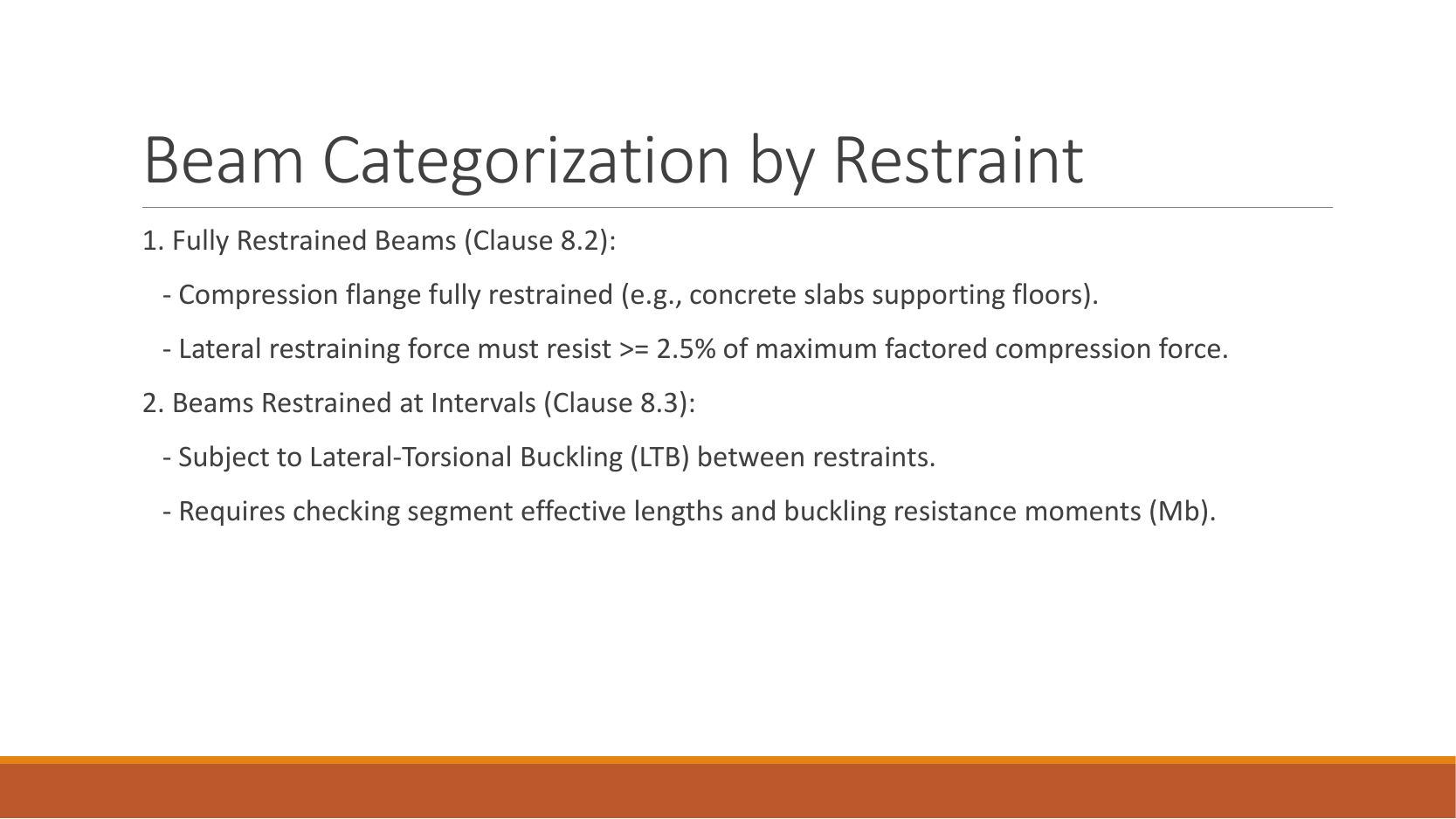
The flange in compression can move sideways and twist the beam. The slide’s restraint-force rule is a strength requirement for the restraint system, not evidence that any slab is automatically an effective restraint. Confirm which flange is in compression and whether the attachment prevents lateral movement/twist.
Study the full explanation and applications.
Animation labA beam bends sideways and twists
Supplement to the original lesson. Enable JavaScript to play, step through calculations and rotate 3D models. The following explanation remains readable offline.
- For the illustrated sagging beam the top flange is compressed.
- The unrestrained compression flange can move sideways while the complete cross-section twists.
- Only effective restraints divide the member into unbraced segments. They do not automatically add vertical supports.
- Use the segment effective length, section properties and matching moment factor. This is an exaggerated mode shape, not a calculated displacement.
PPT/Steel Beam Design L3.pptx · slide 4: Classify the beam
Under major-axis bending the flanges and web have different stress distributions. Use the flange outstand and web from the section table, compare with the correct multiples of , and select the worse class. Do not substitute overall depth for clear web depth .
Study the full explanation and applications.
Animation labWhy thin elements buckle locally
Supplement to the original lesson. Enable JavaScript to play, step through calculations and rotate 3D models. The following explanation remains readable offline.
- The flange outstand and web have different widths, thicknesses and edge support conditions.
- A thinner plate can wrinkle locally before the complete member loses stability.
- Class 1 allows plastic rotation; Class 2 reaches plastic resistance; Class 3 reaches elastic resistance; Class 4 requires effective properties.
- Check every relevant compression element with the supplied limits and stress distribution. The deformation shown is qualitative.
PPT/Steel Beam Design L3.pptx · slide 5: Shear resistance
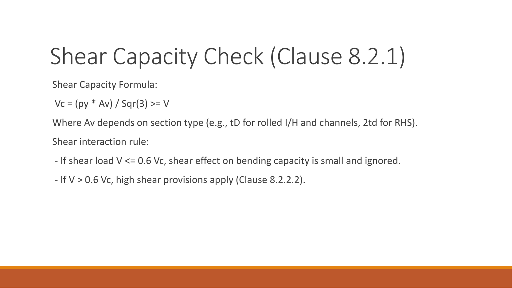
For a rolled I, H or channel under the course major-axis shear model, . Then . Convert to only after multiplying stress by area. If the low-shear bending rule applies; passing alone does not establish low shear.
Study the full explanation and applications.
Animation labSee shear in the web
Supplement to the original lesson. Enable JavaScript to play, step through calculations and rotate 3D models. The following explanation remains readable offline.
- Internal shear keeps the two sides of the cut in vertical equilibrium.
- For the course’s common I-section case, the web provides the principal shear area; use the specified definition.
- A slender web may require a different shear-buckling route before a simple shear-resistance formula is used.
- Use where applicable in the course. Convert N to kN before comparing with design shear.
PPT/Steel Beam Design L3.pptx · slide 6: Low and high shear bending
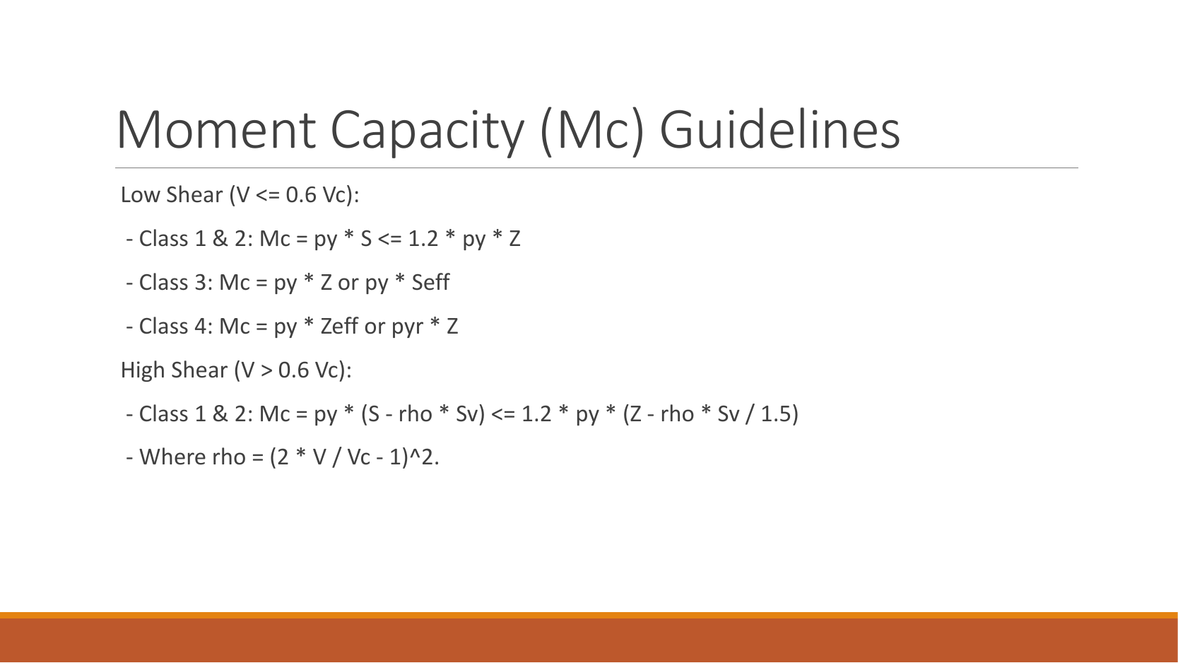
For Class 1/2 at low shear, . Above , reduce bending resistance using the course high-shear formula, with . At , . Use the relevant shear-area term from the full formula, not of the entire bending resistance by guesswork.
Study the full explanation and applications.
Animation labCompression and tension across a section
Supplement to the original lesson. Enable JavaScript to play, step through calculations and rotate 3D models. The following explanation remains readable offline.
- For sagging, the top flange is in compression and the bottom in tension; hogging reverses this.
- Elastic bending stress varies with distance from the neutral axis: .
- The section class governs whether elastic, plastic or effective properties may be used.
- Use the shear at the section under examination; the largest shear elsewhere is not automatically coexistent.
PPT/Steel Beam Design L3.pptx · slide 7: Local web bearing and buckling
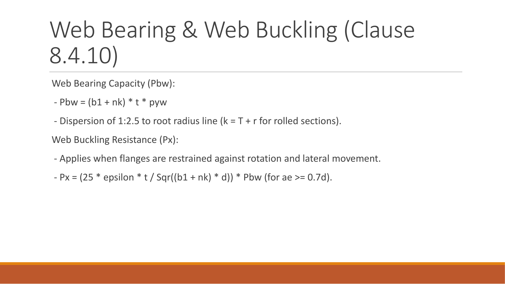
A support reaction or concentrated load presses through a finite bearing length into the web. Bearing and web buckling are separate checks. Identify the stiff bearing length, load position near an end, and lateral restraint. This slide only displays the branch; the full lecture includes the other case. Missing contact dimensions prevent a definite local capacity.
Study the full explanation and applications.
Animation labSpread a concentrated force into the web
Supplement to the original lesson. Enable JavaScript to play, step through calculations and rotate 3D models. The following explanation remains readable offline.
- A concentrated reaction first enters through the bearing/contact region.
- The flange and root geometry spread the force before it enters the web.
- A wider effective bearing region can reduce local stress for the same force.
- End distance, stiff bearing length and restraint conditions must come from the original question. This slider is illustrative only.
PPT/Steel Beam Design L3.pptx · slide 8: LTB factors and effective length
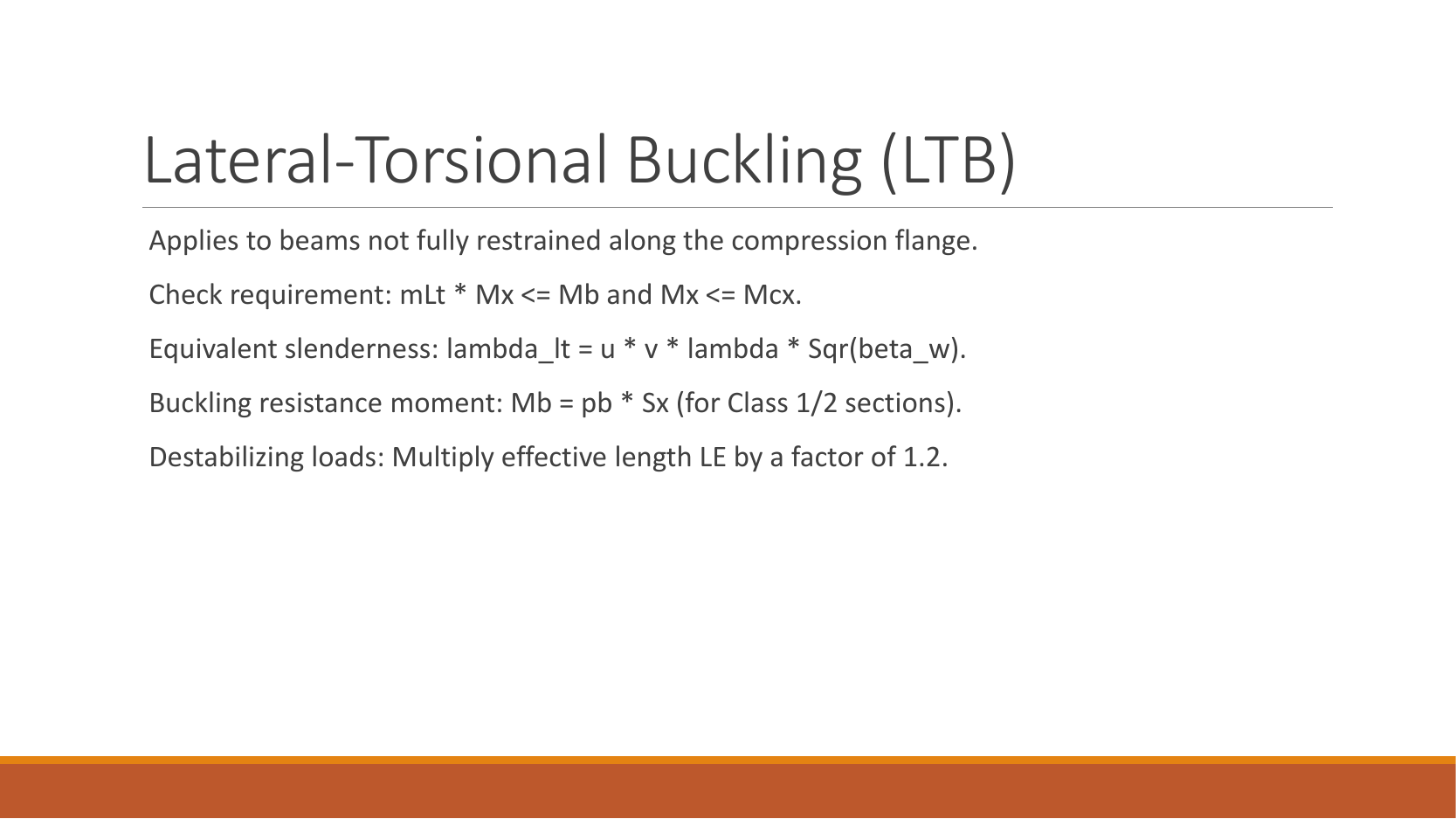
Compute , then and , and read . The slide’s suggestion to multiply destabilizing length by is not a universal rule: use the applicable normal/destabilizing column and actual end-restraint row in the full lecture effective-length rules. Load height and freedom to twist determine applicability.
Study the full explanation and applications.
Animation labA beam bends sideways and twists
Supplement to the original lesson. Enable JavaScript to play, step through calculations and rotate 3D models. The following explanation remains readable offline.
- For the illustrated sagging beam the top flange is compressed.
- The unrestrained compression flange can move sideways while the complete cross-section twists.
- Only effective restraints divide the member into unbraced segments. They do not automatically add vertical supports.
- Use the segment effective length, section properties and matching moment factor. This is an exaggerated mode shape, not a calculated displacement.
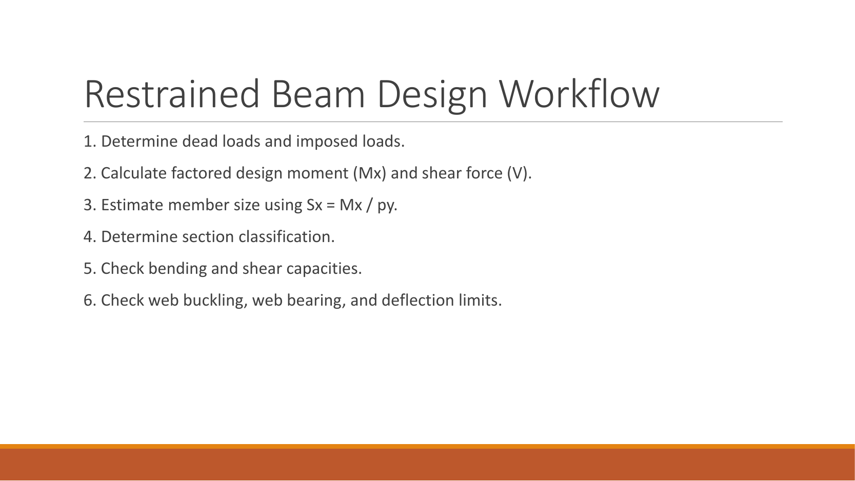
PPT/Steel Beam Design L3.pptx · slide 9: Fully restrained workflow
Resolve loads and reactions; draw the critical moment/shear; choose a trial section; check its class, and ; check local web behaviour; calculate service deflection. State the physical reason LTB is restrained rather than silently omitting it.
Study the full explanation and applications.
Animation labFollow the calculation sequence
Supplement to the original lesson. Enable JavaScript to play, step through calculations and rotate 3D models. The following explanation remains readable offline.
- Locate the load, supports, connection geometry and any stated assumptions.
- Keep given values, table lookups and calculated values distinct; reconcile their units.
- The calculation player steps through the existing expressions in their original order.
- Compare demand with resistance or the relevant limit. Keep missing inputs and conditional conclusions explicit.
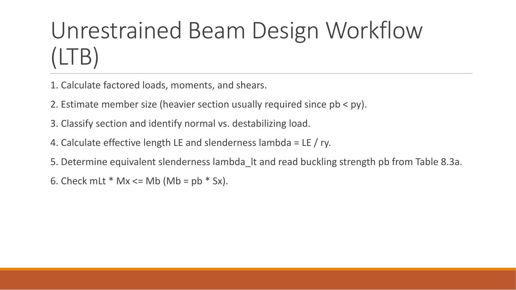
PPT/Steel Beam Design L3.pptx · slide 10: Unrestrained workflow
Divide the beam at effective lateral restraints. For each relevant segment find its maximum moment and moment shape, obtain , calculate effective slenderness and , and compare . The segment with the longest length is not necessarily the governing one.
Study the full explanation and applications.
Animation labA beam bends sideways and twists
Supplement to the original lesson. Enable JavaScript to play, step through calculations and rotate 3D models. The following explanation remains readable offline.
- For the illustrated sagging beam the top flange is compressed.
- The unrestrained compression flange can move sideways while the complete cross-section twists.
- Only effective restraints divide the member into unbraced segments. They do not automatically add vertical supports.
- Use the segment effective length, section properties and matching moment factor. This is an exaggerated mode shape, not a calculated displacement.
PPT/Steel Beam Design L3.pptx · slide 11: Finish with serviceability and a conclusion
Use the stated service load and unamplified elastic stiffness . For central , ; for UDL , . Convert to by ×. State the largest utilization and any incomplete local checks.
Study the full explanation and applications.
Animation labSee stiffness and deflection
Supplement to the original lesson. Enable JavaScript to play, step through calculations and rotate 3D models. The following explanation remains readable offline.
- Use the specified SLS load, span and support arrangement. The demonstrator has a full-span UDL.
- The loaded beam bends; the deformation is exaggerated so its shape can be seen.
- For a simply supported full-span UDL, . Double L with w, E and I unchanged: δ becomes 16 times as large.
- The readout uses , and . Select the finish/support-specific limit from the original table.
PPT/Steel Column Design L4.pptx · slide 1: Column design
A column resists compression, often with bending. A short section can crush; a long member can buckle before reaching material strength. These mechanisms require separate checks.
Study the full explanation and applications.
Animation labA strong slice can belong to an unstable member
Supplement to the original lesson. Enable JavaScript to play, step through calculations and rotate 3D models. The following explanation remains readable offline.
- Combine axial compression and the two bending demands using the specified section resistances.
- The whole member adds effective-length and buckling-curve effects.
- This uses its own moment factor and bending resistance; it is not a copy of the section check.
- Elastic, plastic and buckling resistances are not interchangeable. Read the three original expressions and their first-order/amplified moments.
PPT/Steel Column Design L4.pptx · slide 2: Column learning objectives
Learn restraint interpretation, two-axis slenderness, curve selection, compression resistance and combined axial/bending checks. A single axial capacity is insufficient when the load acts eccentrically.
Study the full explanation and applications.
Animation labWhy thin elements buckle locally
Supplement to the original lesson. Enable JavaScript to play, step through calculations and rotate 3D models. The following explanation remains readable offline.
- The flange outstand and web have different widths, thicknesses and edge support conditions.
- A thinner plate can wrinkle locally before the complete member loses stability.
- Class 1 allows plastic rotation; Class 2 reaches plastic resistance; Class 3 reaches elastic resistance; Class 4 requires effective properties.
- Check every relevant compression element with the supplied limits and stress distribution. The deformation shown is qualitative.
PPT/Steel Column Design L4.pptx · slide 3: Effective length and slenderness
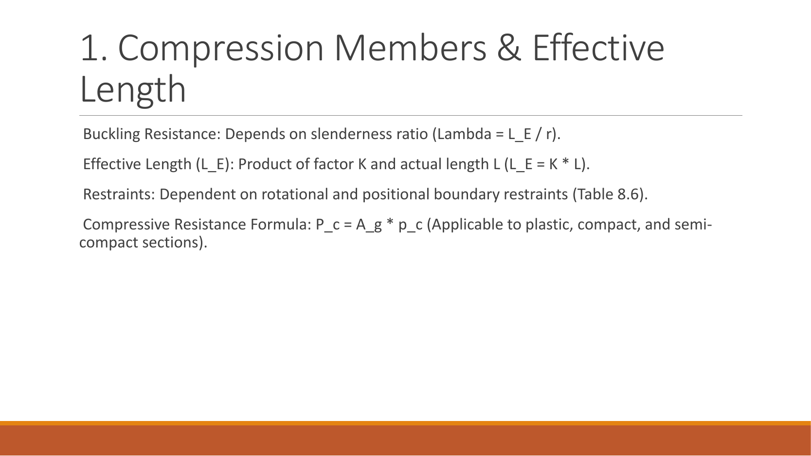
For each axis, and . The dimensionless factor represents the stated end restraint/sway condition. Millimetres must be used in both numerator and denominator. Tying the weak direction reduces only if the tie actually restrains that buckling direction.
Study the full explanation and applications.
Animation labEffective length and buckling axes
Supplement to the original lesson. Enable JavaScript to play, step through calculations and rotate 3D models. The following explanation remains readable offline.
- A column can bow sideways before its section reaches the crushing resistance.
- Each axis has its own radius of gyration and restraint spacing.
- , with compatible length units. A tie affects only the directions it actually restrains.
- Select each buckling curve and compressive strength before forming Pc. The governing axis is determined by resistance, not slenderness alone.
PPT/Steel Column Design L4.pptx · slide 4: Select a strut curve before a number
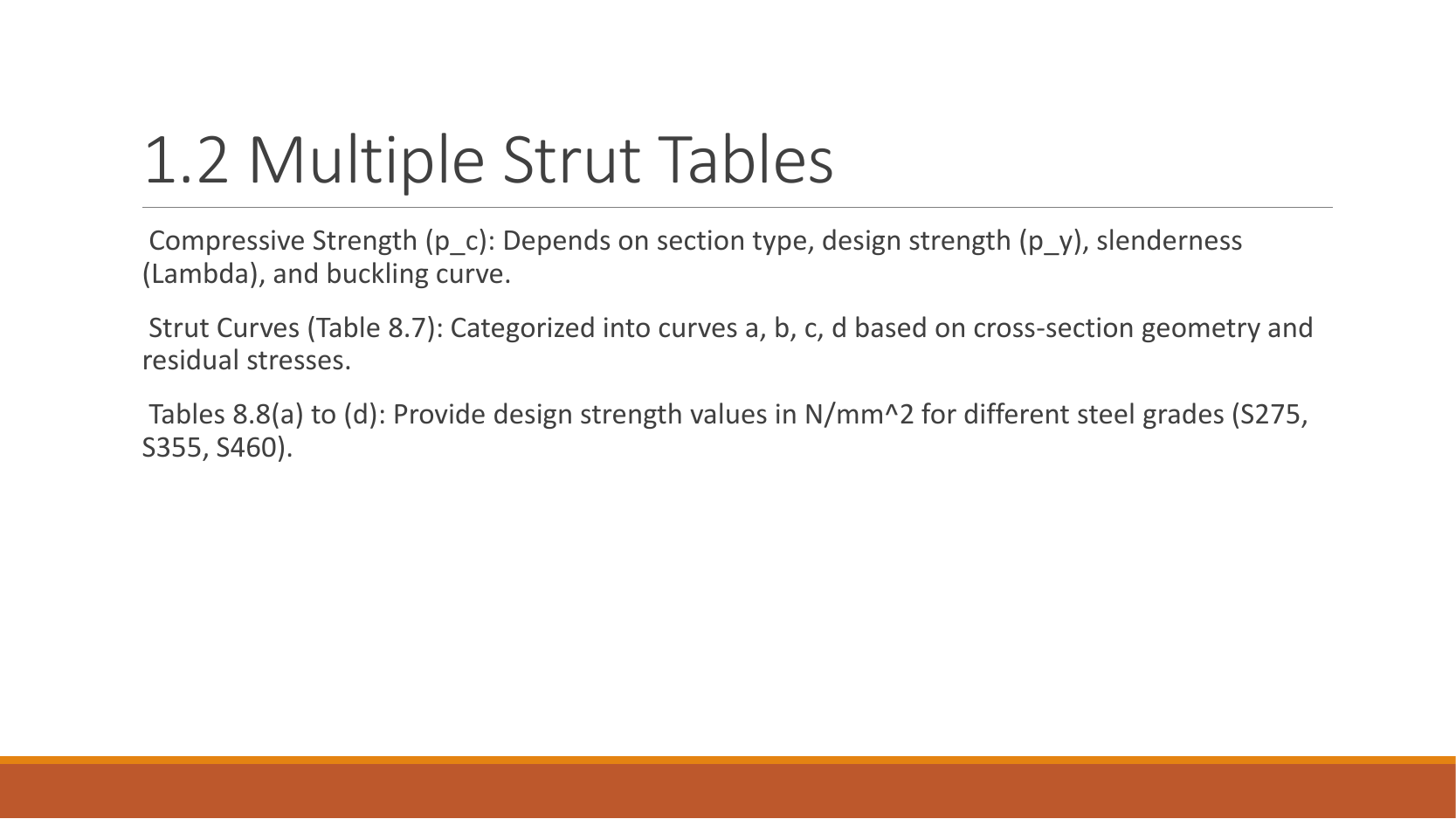
Read Table 8.7 by section type, maximum thickness and buckling axis. A rolled H section with thickness uses curve b about and c about . Then read Table 8.8 using that curve, and slenderness; interpolate between bounding rows.
Study the full explanation and applications.
Animation labEffective length and buckling axes
Supplement to the original lesson. Enable JavaScript to play, step through calculations and rotate 3D models. The following explanation remains readable offline.
- A column can bow sideways before its section reaches the crushing resistance.
- Each axis has its own radius of gyration and restraint spacing.
- , with compatible length units. A tie affects only the directions it actually restrains.
- Select each buckling curve and compressive strength before forming Pc. The governing axis is determined by resistance, not slenderness alone.
PPT/Steel Column Design L4.pptx · slide 5: Section and member interactions
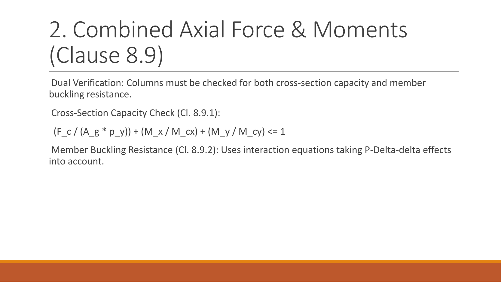
Cross-section interaction combines axial utilization and bending utilizations at the same section. Member equations include reduced compression/LTB resistance and moment factors. Follow the full lecture’s elastic denominators and overbars: compact slide notation can hide whether a moment is first-order or amplified.
Study the full explanation and applications.
Animation labA strong slice can belong to an unstable member
Supplement to the original lesson. Enable JavaScript to play, step through calculations and rotate 3D models. The following explanation remains readable offline.
- Combine axial compression and the two bending demands using the specified section resistances.
- The whole member adds effective-length and buckling-curve effects.
- This uses its own moment factor and bending resistance; it is not a copy of the section check.
- Elastic, plastic and buckling resistances are not interchangeable. Read the three original expressions and their first-order/amplified moments.
PPT/Steel Column Design L4.pptx · slide 6: Frame classification and amplification
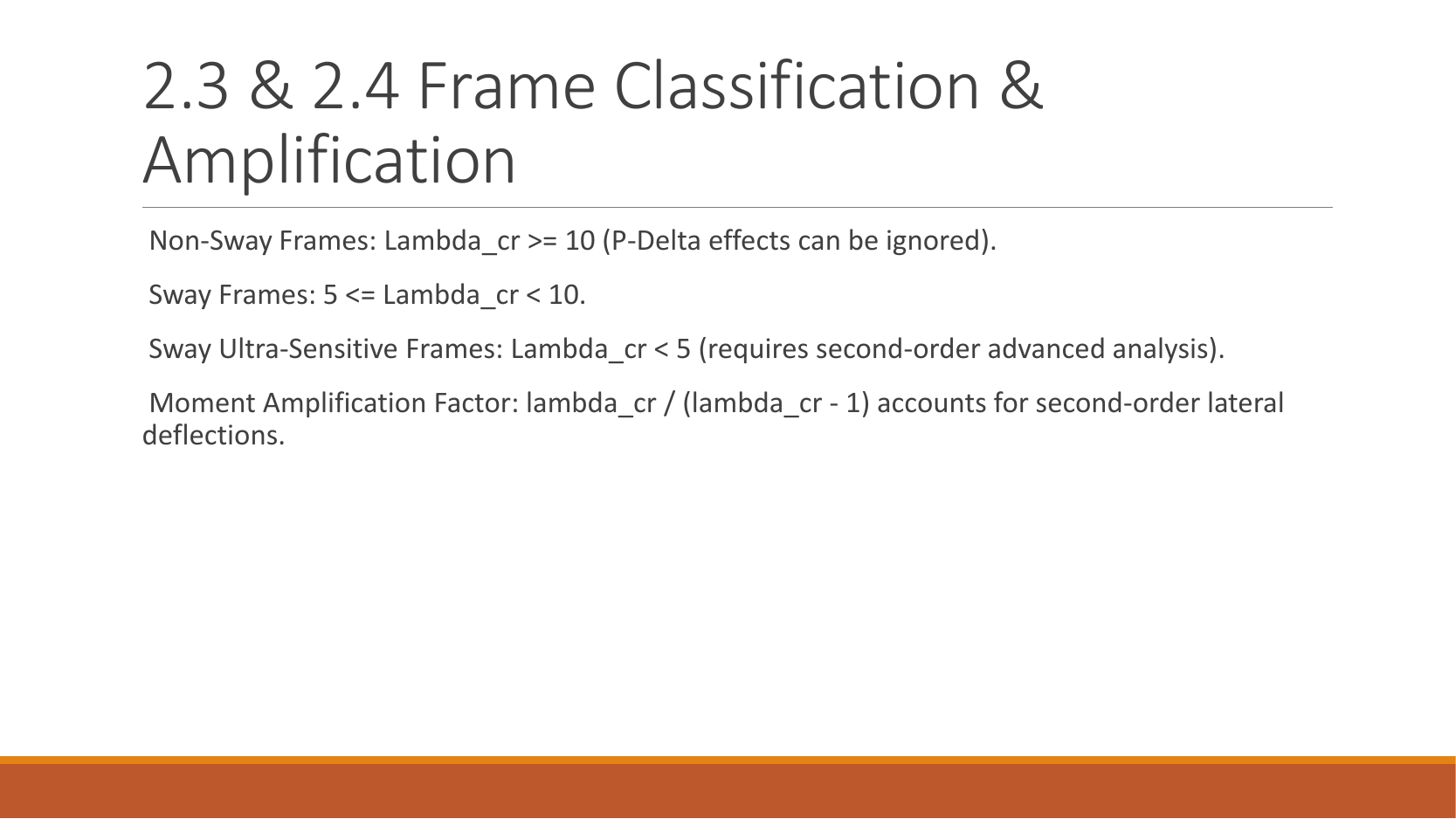
Elastic critical load factor measures proximity to global instability. Use the lecture’s non-sway/sway/ultra-sensitive boundaries and applicable amplification method. If the problem already supplies amplification factors, apply them once to the specified first-order moments; an already amplified must not be amplified again.
Study the full explanation and applications.
Animation labRestraints, sway and imperfections
Supplement to the original lesson. Enable JavaScript to play, step through calculations and rotate 3D models. The following explanation remains readable offline.
- A frame needs a defined path for horizontal force as well as gravity.
- Pinned joints alone do not provide frame moment resistance; sway restraint needs a real structural system.
- Diagonal bracing carries horizontal action through axial forces. This sketch does not assign a numerical frame classification.
- Use the specified imperfection/notional-force model and critical-load criteria. Avoid counting alternative imperfection models twice.
PPT/Steel Column Design L4.pptx · slide 7: Simple construction
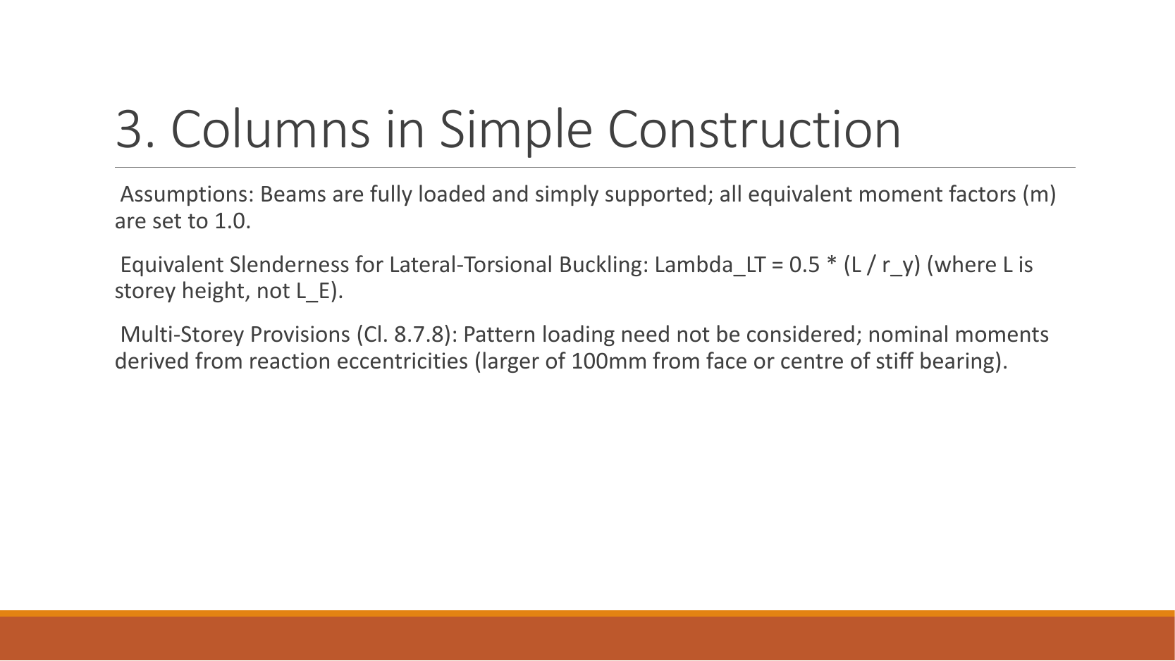
Nominally pinned beams can still deliver eccentric reactions to a column. Calculate reaction×eccentricity and share joint moment according to the prescribed column stiffnesses. For the course simple-construction LTB shortcut, uses actual column length , not the flexural effective length .
Study the full explanation and applications.
Animation labEccentric reactions and stiffness sharing
Supplement to the original lesson. Enable JavaScript to play, step through calculations and rotate 3D models. The following explanation remains readable offline.
- A beam reaction can act away from the column centre even at a nominally pinned beam connection.
- . Opposing reactions can cancel part of the signed moment, while both still add compression.
- The course simple model distributes the joint moment in proportion to of the columns above and below.
- Equal relevant stiffness gives half each. A roof joint with no upper column is a different case.
PPT/Steel Column Design L4.pptx · slide 8: Write both buckling checks accurately
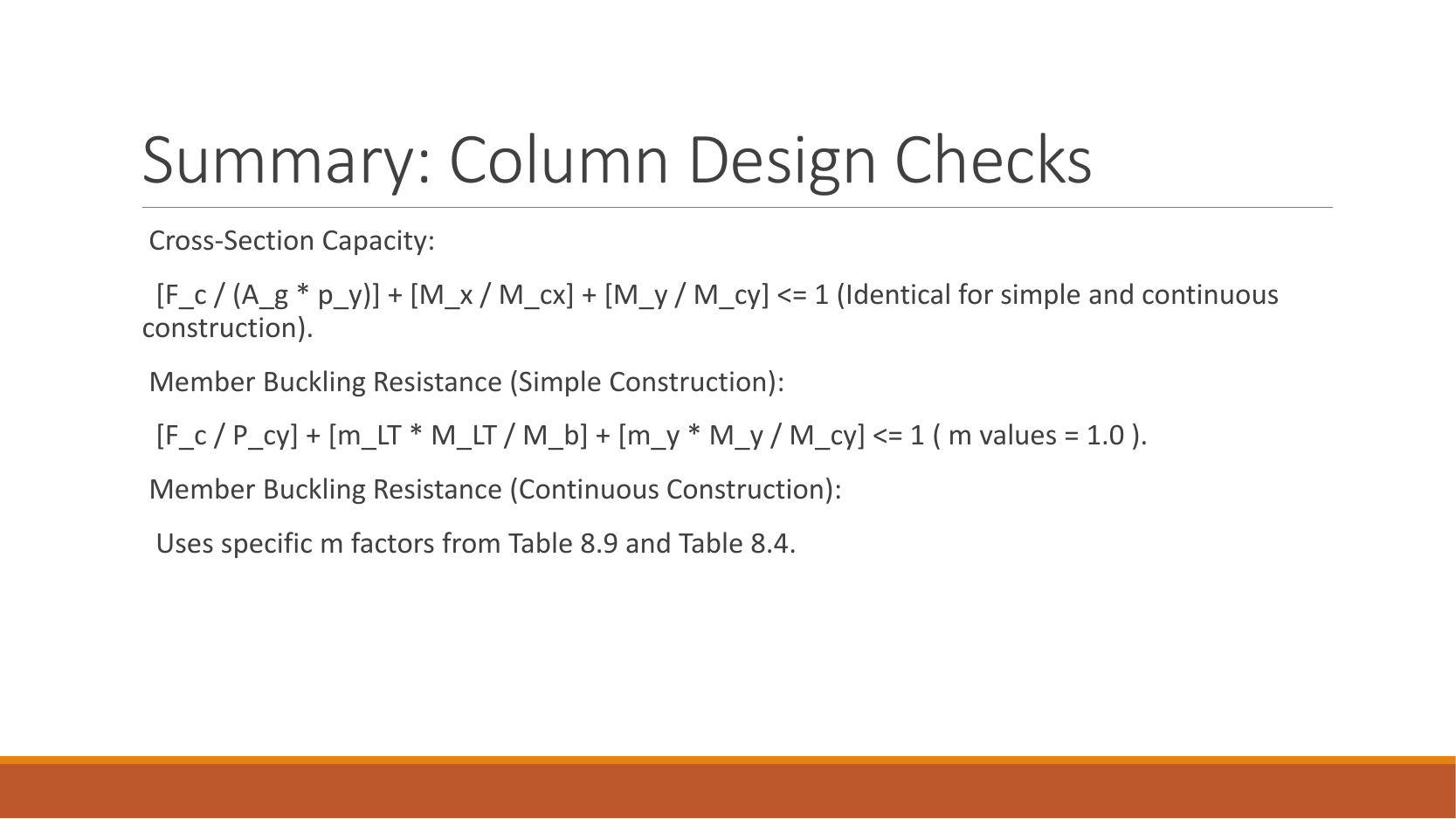
Keep flexural-buckling and LTB interaction equations separate. The full lecture Eq. 8.80 uses amplified bending moments; Eq. 8.81 uses the specified amplified and first-order minor-axis . The slide is a memory aid; use the full derivation to restore subscripts, bars and elastic moment denominators.
Study the full explanation and applications.
Animation labA strong slice can belong to an unstable member
Supplement to the original lesson. Enable JavaScript to play, step through calculations and rotate 3D models. The following explanation remains readable offline.
- Combine axial compression and the two bending demands using the specified section resistances.
- The whole member adds effective-length and buckling-curve effects.
- This uses its own moment factor and bending resistance; it is not a copy of the section check.
- Elastic, plastic and buckling resistances are not interchangeable. Read the three original expressions and their first-order/amplified moments.
PPT/Steel Column Design L4.pptx · slide 9: The worked-example sequence
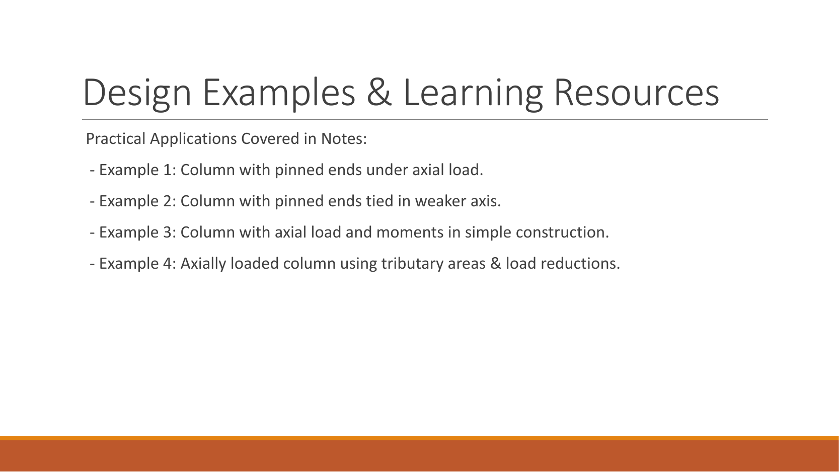
Example 1 teaches axial compression; Example 2 adds a weak-axis tie; Example 3 transfers eccentric beam reactions; Example 4 derives floor loads and reduced imposed load. The full notes also contain Example 5 for combined end moments, which remains required even though this summary omits it.
Study the full explanation and applications.
Animation labEffective length and buckling axes
Supplement to the original lesson. Enable JavaScript to play, step through calculations and rotate 3D models. The following explanation remains readable offline.
- A column can bow sideways before its section reaches the crushing resistance.
- Each axis has its own radius of gyration and restraint spacing.
- , with compatible length units. A tie affects only the directions it actually restrains.
- Select each buckling curve and compressive strength before forming Pc. The governing axis is determined by resistance, not slenderness alone.
PPT/Steel Column Design L4.pptx · slide 10: References and further study
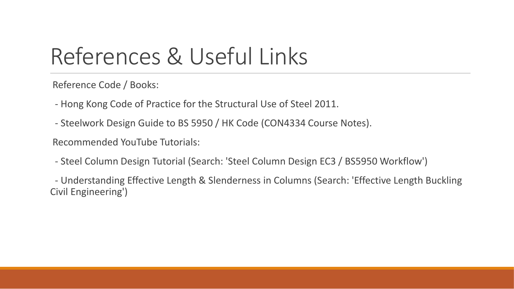
The slide names references and suggests external video searches. This offline course contains the needed teaching locally. When reading outside material, compare code edition, axis labels, yield strength rules and partial factors before using any equation; do not combine Eurocode and supplied HK design expressions.
Study the full explanation and applications.
Animation labRead a table without losing the keys
Supplement to the original lesson. Enable JavaScript to play, step through calculations and rotate 3D models. The following explanation remains readable offline.
- Name the required property: material strength, section property, buckling strength or a moment factor.
- Keep section size, steel grade, thickness band, curve and axis as separate lookup keys.
- , and require different conversion powers. Do not use adjacent columns interchangeably.
- Use bracketing rows within the same valid column. The original page remains the source of all table values.
NOTE.docx · rendered page 1: material and capacities
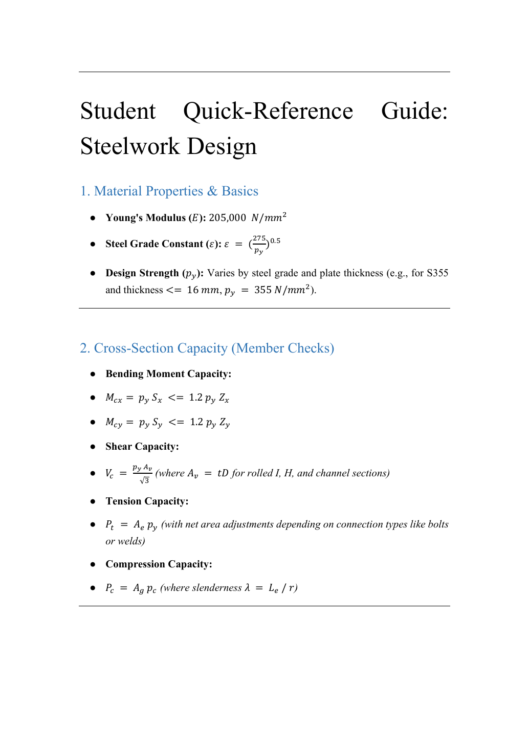
is elastic stiffness. scales classification limits. Read from thickness before calculating . The note lists , but this is the Class 1/2 low-shear rule, not the Class 3/4 rule. uses for the specified rolled sections and shear direction. needs net-area/shear-lag adjustments for connected angles. needs separate curve and slenderness lookups about both axes. Despite the heading “Member Checks”, and alone are cross-section resistances; instability needs additional member checks.
Try it yourself. Why can be less than ?
Reveal answer and reasoning
accounts for member buckling and is normally below ; only describes the material/section strength.
Animation labElasticity, yielding and ductility
Supplement to the original lesson. Enable JavaScript to play, step through calculations and rotate 3D models. The following explanation remains readable offline.
- Stress is force divided by area. Strain measures change in length relative to original length.
- Before yielding, stress is approximately . E controls the elastic slope.
- Further strain includes permanent deformation. Higher yield strength does not by itself increase E.
- Strength, stiffness and ductility answer different questions. This schematic is not a measured stress–strain curve.
NOTE.docx · rendered page 2: deflection and fasteners
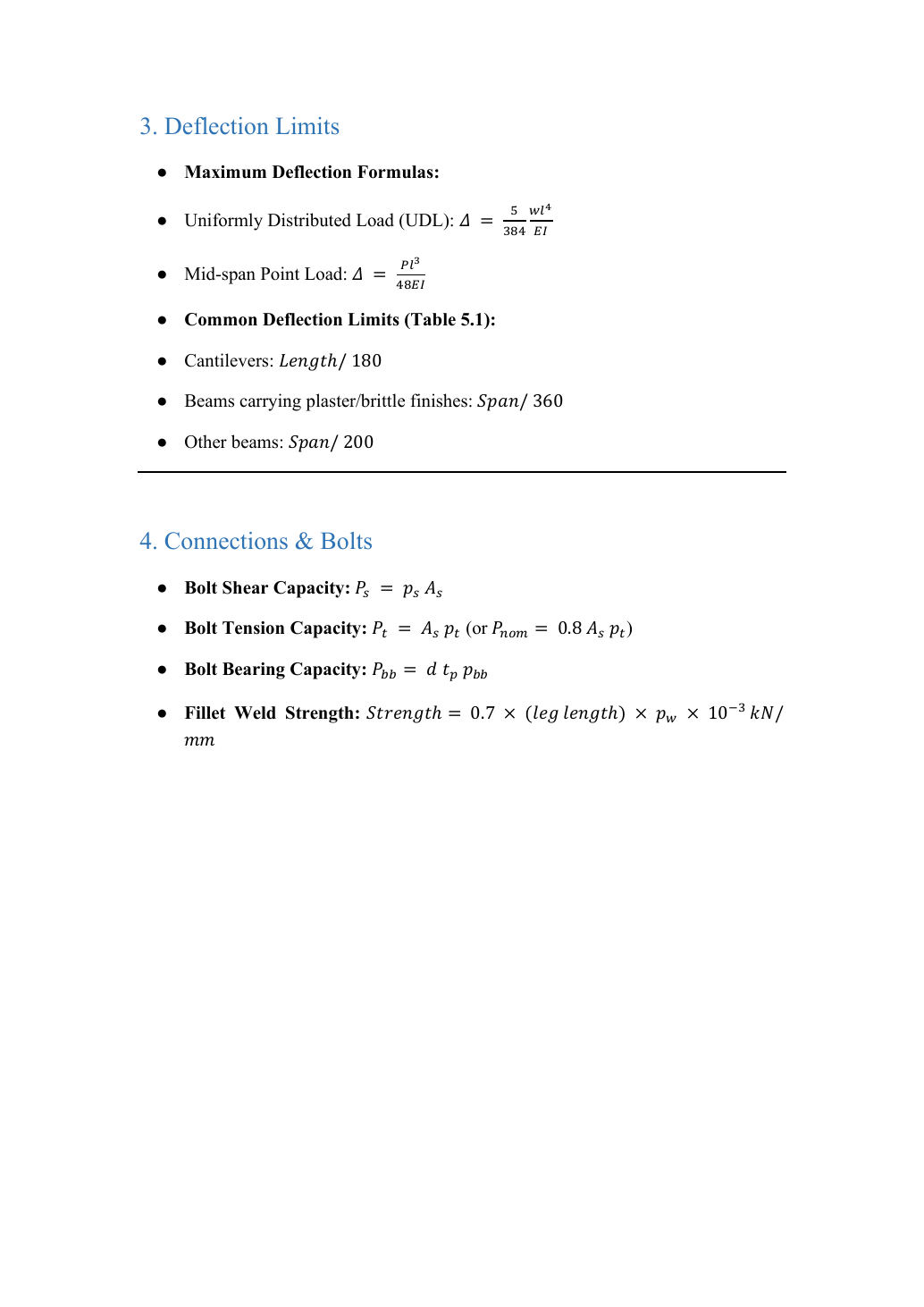
For a simply supported prismatic beam with constant , central-point-load deflection is , and full-span UDL deflection is . The Word note correctly shows for the point load; the separate Data File has a conflicting exponent. Select the service load and limit row, then use consistent and . Bolt is per shear plane; choose shank or thread area from where the plane crosses. is individual tension resistance; is the nominal value used in the specified interaction expression, so the “or” does not permit arbitrary selection. Bolt bearing still requires separate connected-part bearing checks. Weld is strength per millimetre of effective length, not total force.
Try it yourself. A S355/Class 42 fillet has effective length. What direct force can it carry?
Reveal answer and reasoning
; resistance, subject to detailing and parent-metal checks.
Animation labFrom fillet leg to effective throat
Supplement to the original lesson. Enable JavaScript to play, step through calculations and rotate 3D models. The following explanation remains readable offline.
- An equal-leg fillet between perpendicular plates has an approximately right-triangular section.
- For this geometry, throat . It is shorter than the leg.
- Effective resisting area = . With here, capacity per length is .
- Use the course end allowances, minimum size and length rules; increasing the geometric length alone does not resolve every detailing check.
Animation labSee stiffness and deflection
Supplement to the original lesson. Enable JavaScript to play, step through calculations and rotate 3D models. The following explanation remains readable offline.
- Use the specified SLS load, span and support arrangement. The demonstrator has a full-span UDL.
- The loaded beam bends; the deformation is exaggerated so its shape can be seen.
- For a simply supported full-span UDL, . Double L with w, E and I unchanged: δ becomes 16 times as large.
- The readout uses , and . Select the finish/support-specific limit from the original table.