2014–2019 · Reference answers
2017-05-19 — column answer
Check 254 × 254 × 107 UC under combined compression and biaxial bending.
Independent teaching answer, not an official solution or marking scheme.
Printed marks are retained.
Read the source conditions beside each result.
Strategy and prerequisites
A strong cross-section can belong to an unstable member
A column carries axial compression and bending. Explain why more than one check is required.
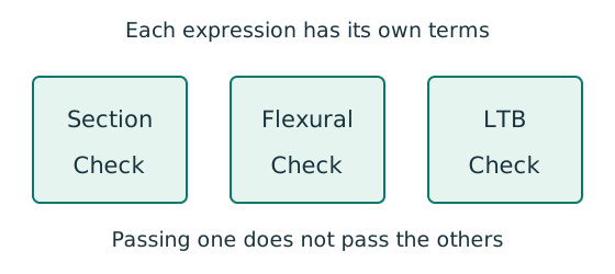
Prediction, then explanation. At fixed moments and resistances, increasing compression increases utilisation. A section pass cannot remove the length-dependent instability checks.
Separate cross-section, flexural-buckling and LTB interaction equations. Use each equation’s own denominators and first-order or amplified moments.
is a section axial resistance. is a member compression resistance. Elastic and prescribed are different bending denominators.
Scope. Preserve the course barred-moment definitions and Eq. 8.81 convention. Do not substitute plastic moduli into an elastic denominator.
Check and takeaway. Report each requested utilisation and the governing check. The largest properly calculated ratio identifies the closest limit.
Change the ruler, keep the quantity
A section table uses centimetres, but the strength calculation uses millimetres. The numbers must describe the same section.
Prediction, then explanation. Would every property increase by ten? No. The exponent determines how many factors of ten are needed.
First identify the physical quantity. Next convert each length factor. Keep force and length conversions separate when converting a moment.
Here n is the length exponent: 2 for area, 3 for section modulus and 4 for second moment of area.
Scope. Changing units changes neither the load nor the section. A conversion factor cannot repair a formula for the wrong physical quantity.
Check and takeaway. Illustration: . The fourth power belongs to the unit, not the number 2.
Apply the reasoning to this section’s data and conditions
Units: 1 kN = 1,000 N; 1 m = 1,000 mm; 1 cm³ = 1,000 mm³; 1 cm⁴ = 10,000 mm⁴.
Demand is the load effect.
Resistance is the permitted capacity for the selected failure mode.
Compare matching units.
Physical interpretation and limits
A section is one slice of the column; buckling concerns the whole long member.
Three passing checks are needed, just as a strong ruler can still bend sideways when pushed at its ends.
Biaxial column checks [30 marks]
Use the same mechanism: A strong cross-section can belong to an unstable member. At fixed moments and resistances, increasing compression increases utilisation. A section pass cannot remove the length-dependent instability checks.
Apply the reasoning to this section’s data and conditions
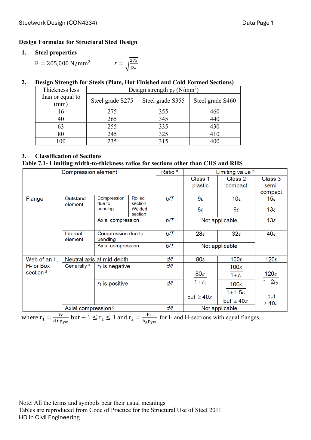
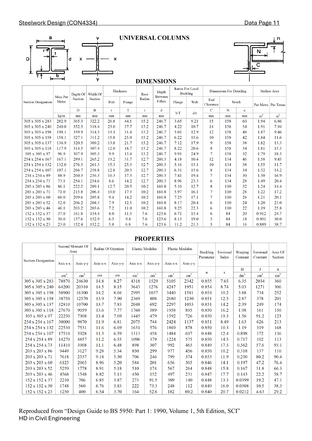
Exact UC row: 254 × 254 × 107.
A is gross area, r radius of gyration, Z elastic modulus, S plastic modulus.
Convert the tabulated radii from cm to mm.
Do not use nominal section size as a radius.
The conservative Class 1 web bound 40ε is valid for the course combined-stress formula because its axial stress parameter is bounded by one.
Check the flange separately.
Use the worse class.
Overall Class 1.
The horizontal x–x axis passes through the web; y–y is vertical on the plan.
A vertical drawing offset creates Mx.
A horizontal offset creates My.
All point forces are axial compression.
Opposite offsets give opposite moments.
Sum all axial forces, but share the joint moments equally between the equally stiff upper and lower columns.
| Force (kN) | Horizontal x (mm) | Vertical y (mm) |
|---|---|---|
| 400 | 100 | 0 |
| 200 | 0 | 150 |
| 300 | 0 | -180 |
At a section, combine compression and amplified bending using capped plastic resistances for Class 1/2.
All three fractions are dimensionless.
PASS
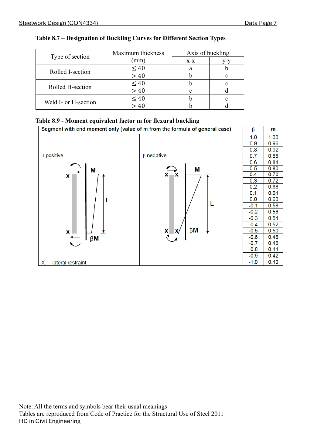
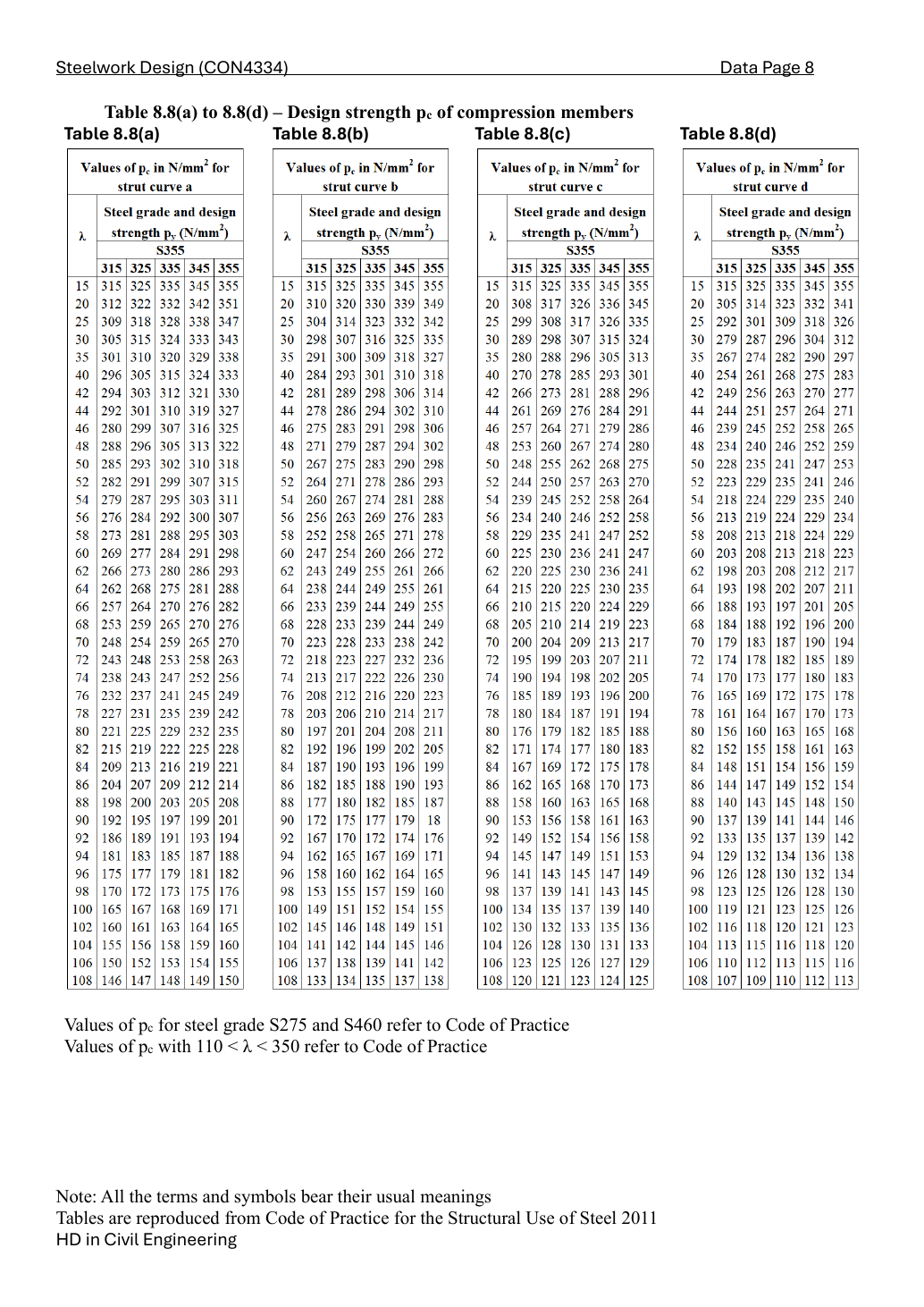
Rolled UC with flange thickness 20.5 mm ≤ 40 mm: curve b about x and curve c about y.
Use py = 345 N/mm² in both tables.
Linear interpolation uses adjacent slenderness rows, not the nearest section size.
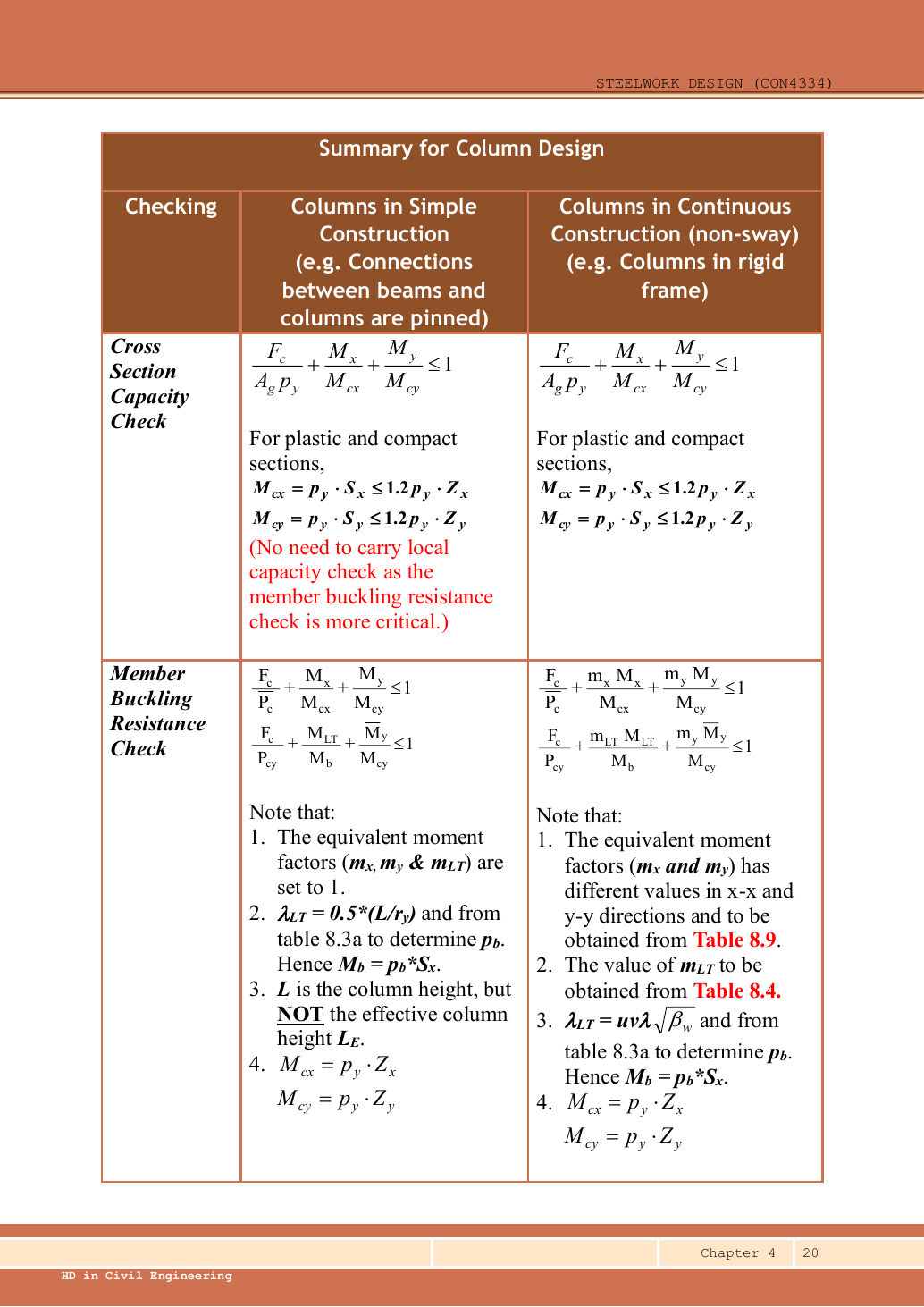
All moment factors are given as one.
The simple-construction LTB slenderness uses ACTUAL storey height, not the compression effective length.
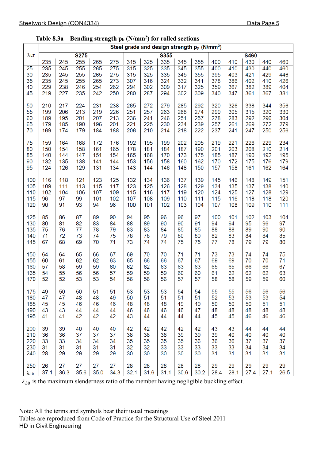
Table 8.3: py 345 column, λLT rows 30 to 35.
Member interaction uses ELASTIC moduli in the ordinary bending denominators.
First equation: smaller axial buckling resistance and amplified moments.
Second equation: Pcy and MLT, with first-order minor-axis moment.
PASS
PASS
Result and concise exam wording — key result lines
All three checks: PASS under the stated model.
Procedure and common mistakes
Compression acts on the displaced shape
A compressed member moves away from its initial load line. Explain why the bending moment can increase.
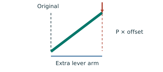
Prediction, then explanation. At fixed axial force, a larger offset creates a larger additional moment. This can further increase the displacement.
Force acting through an offset forms a moment. Second-order analysis includes that changed geometry in equilibrium.
P is axial force. Δ and δ are the relevant perpendicular displacements. Consistent force and length units give moment units.
Scope. Use the amplification or analysis method stated for the frame. Do not amplify an already amplified moment a second time.
Check and takeaway. Zero offset removes this additional moment in the ideal sketch. Real design may still require imperfections and code checks.
Vertical bending can trigger sideways motion
A beam has enough local bending resistance. Check whether its compression flange can move sideways and twist.
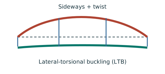
Prediction, then explanation. Adding a valid lateral restraint shortens a stability segment. It need not change the beam’s vertical reaction or moment diagram.
Identify the compressed flange and effective restraints. Calculate the specified slenderness, read buckling strength and compare resistance with the segment demand.
LE and ry use the same length unit. pb uses N/mm²; Sx uses mm³; Mb uses N·mm. mLT is dimensionless.
Scope. Use the specified section class, effective-length branch and loading condition. Load height alone does not prove a destabilizing case.
Check and takeaway. Removing a lateral restraint requires a new segment stability check. The old shorter-segment result cannot establish the longer segment’s adequacy.
Check buckling about both axes
Determine which buckling direction limits the compressed member.
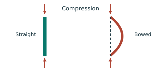
Prediction, then explanation. At fixed radius, longer effective length raises slenderness. The supplied buckling curve generally gives lower compressive strength.
Calculate slenderness about each axis. Select each axis’s curve from section type and thickness. Then obtain and compare the two compressive resistances.
Effective lengths and radii use mm. pc is compressive strength in N/mm²; Ag is gross area in mm²; Pc is in N.
Scope. Do not select the governing axis using radius alone. Effective length and buckling curve can differ. A combined column also needs interaction checks.
Check and takeaway. A short-section yield resistance is not the same as long-member buckling resistance. Keep py and pc distinct.
Apply the reasoning to this section’s data and conditions
Identify the model → axes and actions → class → section → both strut curves → LTB → both member equations.
Do not halve axial load, swap x/y moduli, replace the given effective length with the actual height, or amplify MLT twice.
Explained variant — invented example
Use the same mechanism: A strong cross-section can belong to an unstable member. At fixed moments and resistances, increasing compression increases utilisation. A section pass cannot remove the length-dependent instability checks.
Use the same mechanism: Check buckling about both axes. At fixed radius, longer effective length raises slenderness. The supplied buckling curve generally gives lower compressive strength.
Apply the reasoning to this section’s data and conditions
Invented variant: axial load increases by 100 kN, moments and class unchanged.
How does each utilisation change?
Hint
Only the axial-force numerator changes in this stated variant.