Formula selection and fully worked lookup tables
Open “Animation lab” beside a teaching step for a visual explanation or a walkthrough of its original expressions. Models are illustrative; source answers remain unchanged.
Use this as a formula-selection and table-reading lesson. All tables below are supplied course sources, retained locally. Equations are explained in the method chapters and applied in the worked examples. No external standard or unprovided clause is substituted.
Units and a reliable lookup routine
| Quantity | Source unit → calculation unit |
|---|---|
| Force | |
| Moment | ; |
| Area | |
| Section modulus | |
| Second moment of area | |
| Radius of gyration | |
| Line load | |
| Stress |
- Name the physical check and identify which table is applicable.
- Write section designation, grade, thickness, axis and restraint assumptions.
- Write the exact source, table title, column heading and bounding row numbers.
- Show interpolation fraction and substitution with units.
- Check the result lies between the two table values; check higher slenderness has not accidentally increased resistance.
Animation labUnits and powers
Supplement to the original lesson. Enable JavaScript to play, step through calculations and rotate 3D models. The following explanation remains readable offline.
- Force, length and stress must use compatible units before substitution.
- . An area has two length factors, so .
- A section modulus has ; second moment of area has . Use and for cm to mm.
- . Divide by to express that moment in .
Data File 1: Material strength and classification
Read the steel-grade heading, then the first thickness upper bound that contains the actual governing thickness. For S355, uses ; uses the row, . Calculate . In Table 7.1 select flange/web, rolled/welded and bending/compression stress pattern; compare and to the class limits. Take the worse element class. The compression stress parameter is bounded between and ; do not use a pure-bending web limit for uniform compression.
Full method and worked application.
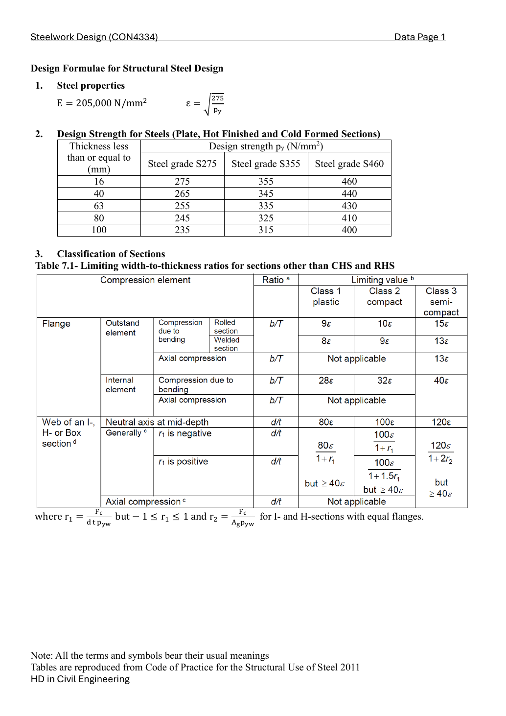
Source labels and selectable formulas: Design Formulae for Structural Steel Design; Steel properties, ,. The following values are retained from the source table, not measured from image scale.
| Upper thickness limit () | S275 | S355 | S460 |
|---|---|---|---|
| Compression element / stress pattern | Ratio | Class 1 | Class 2 | Class 3 |
|---|---|---|---|---|
| Hot-rolled flange outstand in compression from bending | ||||
| Welded flange outstand in compression from bending | ||||
| Flange outstand under axial compression | Not applicable | Not applicable | ||
| Internal flange element in compression from bending | ||||
| Internal flange element under axial compression | Not applicable | Not applicable | ||
| I/H/box web with neutral axis at mid-depth | ||||
| General web case, negative | ; the source notes | , and | ||
| General web case, positive | ; the source notes | , and | , and | |
| Web under axial compression | Not applicable | Not applicable | , and |
Original expressions below the table: , but ; for equal-flange I/H-sections, . The source merged Class 1 cell prints , whereas Classes 2/3 print . This distinction is retained without silently changing the equality boundary. Superscripts a, b, c and d are footnote markers; the page does not expand every note, so use the full course classification table. The footer states that symbols have their usual meanings, the table is extracted from the Hong Kong 2011 steel code, and the course is HD in Civil Engineering.
Animation labRead a table without losing the keys
Supplement to the original lesson. Enable JavaScript to play, step through calculations and rotate 3D models. The following explanation remains readable offline.
- Name the required property: material strength, section property, buckling strength or a moment factor.
- Keep section size, steel grade, thickness band, curve and axis as separate lookup keys.
- , and require different conversion powers. Do not use adjacent columns interchangeably.
- Use bracketing rows within the same valid column. The original page remains the source of all table values.
Data File 2: Beam, tension and compression equations
Class 1/2 low-shear ; . Simply supported deflection: full-span UDL ; central point load . For LTB use , then compare . Angle tension uses the appropriate bolted/welded, single/double reduction of outstanding-leg area . Compression uses , with read for each axis. The point-load exponent printed on this Data File page is : this is dimensionally wrong; the lecture, Word note and 2023 data show .
Full method and worked application.
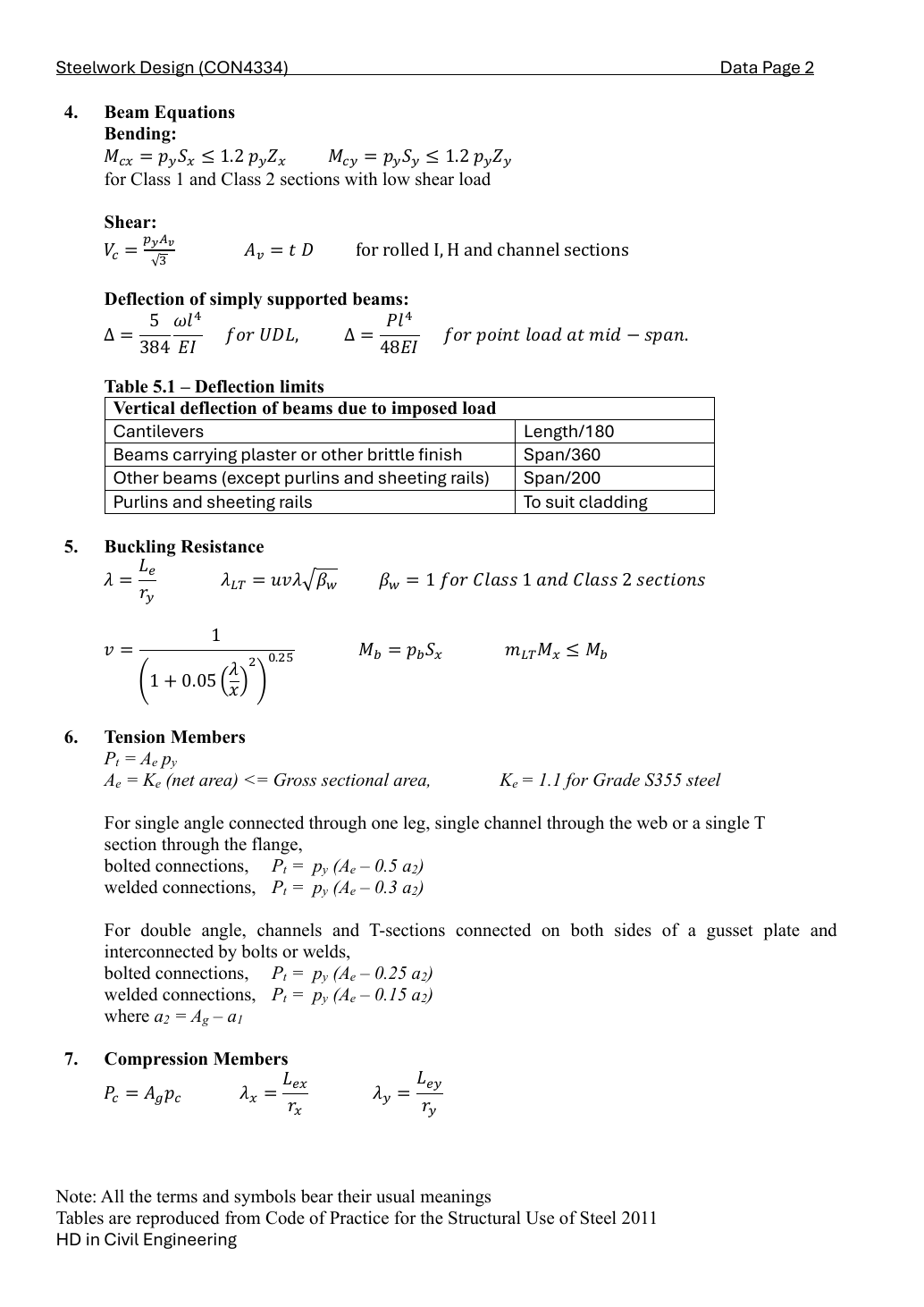
Source item 4, Beam Equations. Class 1/2 at low shear: ,. Shear resistance ; for hot-rolled I, H and channel sections, . The source simply supported UDL deflection is ; for a midspan point load, the source prints . The fourth power in the latter is an identified error; the source image is retained. The correct cubic formula is given above. The source lower-case , and this lesson's , correspond respectively to span and UDL intensity.
Table 5.1 refers to vertical deflection caused by imposed load: cantilever limit ; beams carrying plaster or other brittle finishes ; other beams excluding purlins and sheeting rails ; purlins and sheeting rails must meet cladding requirements.
Item 5, Buckling Resistance: ,; for Classes 1/2, ; ,,. Here is the torsional index, not a position coordinate.
Item 6, Tension Members: ,; for S355, . A single angle connected through one leg, single channel through its web or single tee through its flange uses the following for a bolted connection: ; welded: . For paired angles/channels/tees on opposite sides of a gusset, interconnected by bolts or welds, the bolted expression is ; welded: ; .
Item 7, Compression Members: ,,. The lower-case effective-length subscript and are retained from the source. Symbols and applicability must agree with the complete method. The footer identifies the Hong Kong 2011 steel code as the table source.
Animation labCompression and tension across a section
Supplement to the original lesson. Enable JavaScript to play, step through calculations and rotate 3D models. The following explanation remains readable offline.
- For sagging, the top flange is in compression and the bottom in tension; hogging reverses this.
- Elastic bending stress varies with distance from the neutral axis: .
- The section class governs whether elastic, plastic or effective properties may be used.
- Use the shear at the section under examination; the largest shear elsewhere is not automatically coexistent.
Data File 3: Column interactions and weld groups
The compact column equations omit information visible in the full lecture, including elastic denominators and amplified-moment notation. Use the linked column method to restore these details. For a rectangular four-sided line weld of width and height : , , and , all line inertias in . At coordinates , torsional components are and in when is . Add direct components before taking the resultant. These formulas do not describe a missing-side weld.
Full method and worked application.
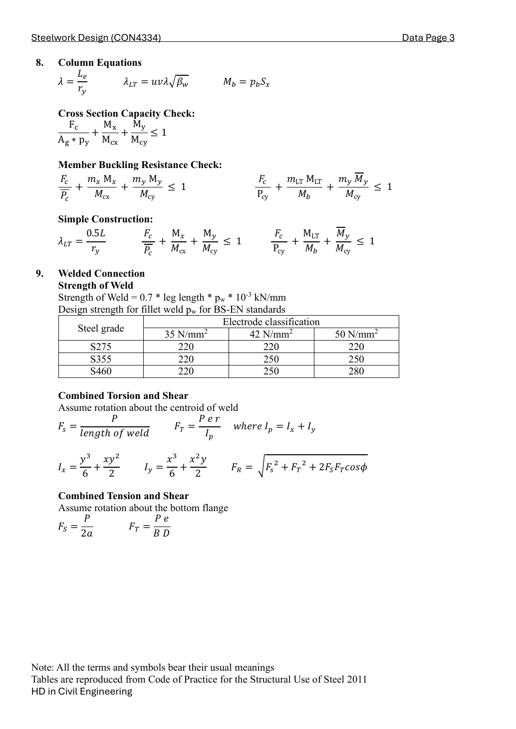
Item 8, Column Equations. The following faithfully reproduce the data sheet's shorthand, which does not replace the full lecture: ,,. Section check: .
Original member expressions: ; . Original simple-construction expression: ; ; . Denominators and overbar positions on this page do not all match the full lecture. In a solution, use the complete method linked above to distinguish elastic moment resistance and amplified/first-order moments; do not assume they are interchangeable.
Item 9, Welded Connection. Original resistance per millimetre of weld length: ; leg length means weld leg, entered in , with is measured in is substituted.
| Steel grade | 35 | 42 | 50 |
|---|---|---|---|
| S275 | |||
| S355 | |||
| S460 |
Combined torsion and shear, assuming rotation about the weld centroid: ,,; ,; . In these two inertia expressions, , are full rectangle width and height, corresponding to , above, not the earlier corner coordinates; corresponds to .
Combined tension and shear: the source assumes rotation about the bottom flange and gives ,. This data sheet has no sketch defining where , , is measured. Establish it from the corresponding question or lecture geometry; do not infer it from this page. Here is tension, different from the torsional component in the previous paragraph. The footer identifies the Hong Kong 2011 steel code as the source.
Animation labA strong slice can belong to an unstable member
Supplement to the original lesson. Enable JavaScript to play, step through calculations and rotate 3D models. The following explanation remains readable offline.
- Combine axial compression and the two bending demands using the specified section resistances.
- The whole member adds effective-length and buckling-curve effects.
- This uses its own moment factor and bending resistance; it is not a copy of the section check.
- Elastic, plastic and buckling resistances are not interchangeable. Read the three original expressions and their first-order/amplified moments.
Data File 4: Ordinary bolts and connected-part bearing
Choose the nominal diameter row; use tensile area for tension and thread shear, shank area only for an unthreaded shear plane. Grade selects ,,. For double shear count two planes, but bearing depends on the actual contacting plate thickness. Check connected-part bearing with the diameter term, end-distance term and clear-ligament/bolt-tensile cap. For eccentric groups use the correct centroid or rotation pivot. The combined shear/tension limit is plus individual checks, not a replacement for them.
Full method and worked application.
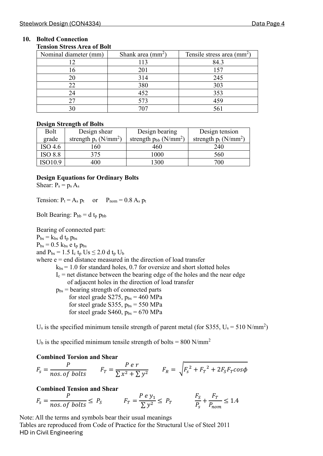
| Nominal diameter () | Shank area () | Tensile stress area () |
|---|---|---|
| Bolt grade | Shear | Bearing | Tension |
|---|---|---|---|
| ISO 4.6 | |||
| ISO 8.8 | |||
| ISO 10.9 |
Ordinary bolts: shear ; tension ; the specified interaction expression instead uses nominal value ; bolt bearing . For bearing of connected parts, the source lists in order , , and . Take the governing applicable limit; do not add the resistances.
is end distance measured along the load-transfer direction. Standard holes: ; oversized and short-slotted holes: . is the clear distance in the load-transfer direction from a hole's bearing edge to the nearest edge of the adjacent hole. Connected-part bearing strengths: for S275, ; for S355, ; for S460, . The specified minimum ultimate tensile strength of the parent metal is ; for S355, . The page lists bolt ; that value corresponds to the course Grade 8.8 examples, not every other bolt grade in the table above.
Combined torsion and shear: ,,. Combined tension and shear: ,,. In the final individual tension limit, the source uses an upper-case subscript , while the tension definition above uses . The original lettering is retained and its correspondence identified. The two uses of likewise mean torsional component and tension respectively. Measure coordinates from the applicable centroid/rotation centre. The footer identifies the Hong Kong 2011 steel code as the source.
Animation labCount the bolt shear planes
Supplement to the original lesson. Enable JavaScript to play, step through calculations and rotate 3D models. The following explanation remains readable offline.
- Load must cross an interface between the connected plates.
- A lap joint gives one shear plane through a bolt.
- A symmetric double-cover joint may provide two shear planes. Count load-transfer interfaces, not just visible plates.
- Use the source’s area and shear strength. Then check bearing, plate resistance and detailing separately.
Data File 5: Table 8.3a: LTB bending strength
First calculate , not merely . Choose the column within the steel grade. Locate its two surrounding rows, interpolate linearly and multiply by . If the input exceeds available rows, obtain the applicable source table rather than extrapolating. For a value below the first printed row , this site conservatively uses row ; it never makes exceed . at the bottom indicates the negligible-buckling range and is not an extra multiplier.
Full method and worked application.
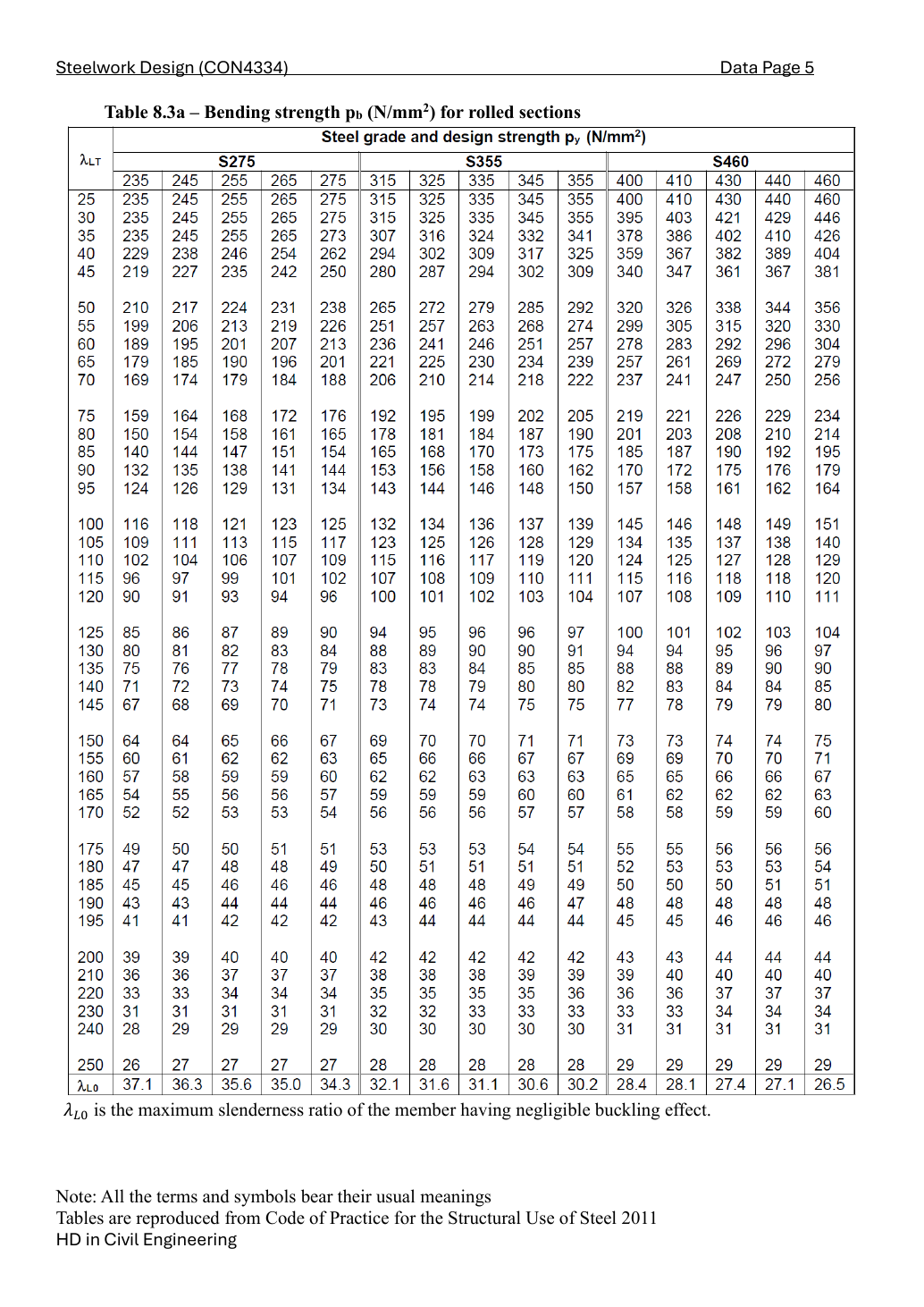
Source heading: bending strength of hot-rolled sections , in ; rows give . For S275, the columns are, in order, ; for S355, ; for S460, , with the same units. The bottom row gives the maximum slenderness at which member-buckling effects can be neglected. In the same column order, S275: ; S355: ; S460: .
Original website transcription differences:The existing two-column HTML table below preserves the original website record. Four rows in its 355 column are incorrect; use the corrections here or the source image above. Every row in the 345 column matches this image. The columns and headings have been rechecked against the original table embedded in the PDF; the adjacent 400 column has not been read as the 355 column. Tutorial 3 Q3 and 2023 BQ4 use rows //, whose original values // are correct. The earlier mistaken corrections to those two questions have been withdrawn. Neither question uses the four rows below.
| Original website value (incorrect) | Source-image value (use this) | |
|---|---|---|
Interpolation fraction .
| at py 345 () | at py 355 () | |
|---|---|---|
Animation labA beam bends sideways and twists
Supplement to the original lesson. Enable JavaScript to play, step through calculations and rotate 3D models. The following explanation remains readable offline.
- For the illustrated sagging beam the top flange is compressed.
- The unrestrained compression flange can move sideways while the complete cross-section twists.
- Only effective restraints divide the member into unbraced segments. They do not automatically add vertical supports.
- Use the segment effective length, section properties and matching moment factor. This is an exaggerated mode shape, not a calculated displacement.
Data File 6: Tables 8.4a/b: equivalent LTB moment
Match the whole unrestrained segment to the sketch, including its end moments and intermediate loads. A simply supported central point load uses ; a full-span UDL uses the supplied shortcut. For a general diagram use the absolute quarter-point ordinates in Table 8.4b and its minimum . If a more accurate quarter-point result differs slightly from a shortcut, state which prescribed method you used. Cantilevers without intermediate restraint use under the supplied table.
Full method and worked application.
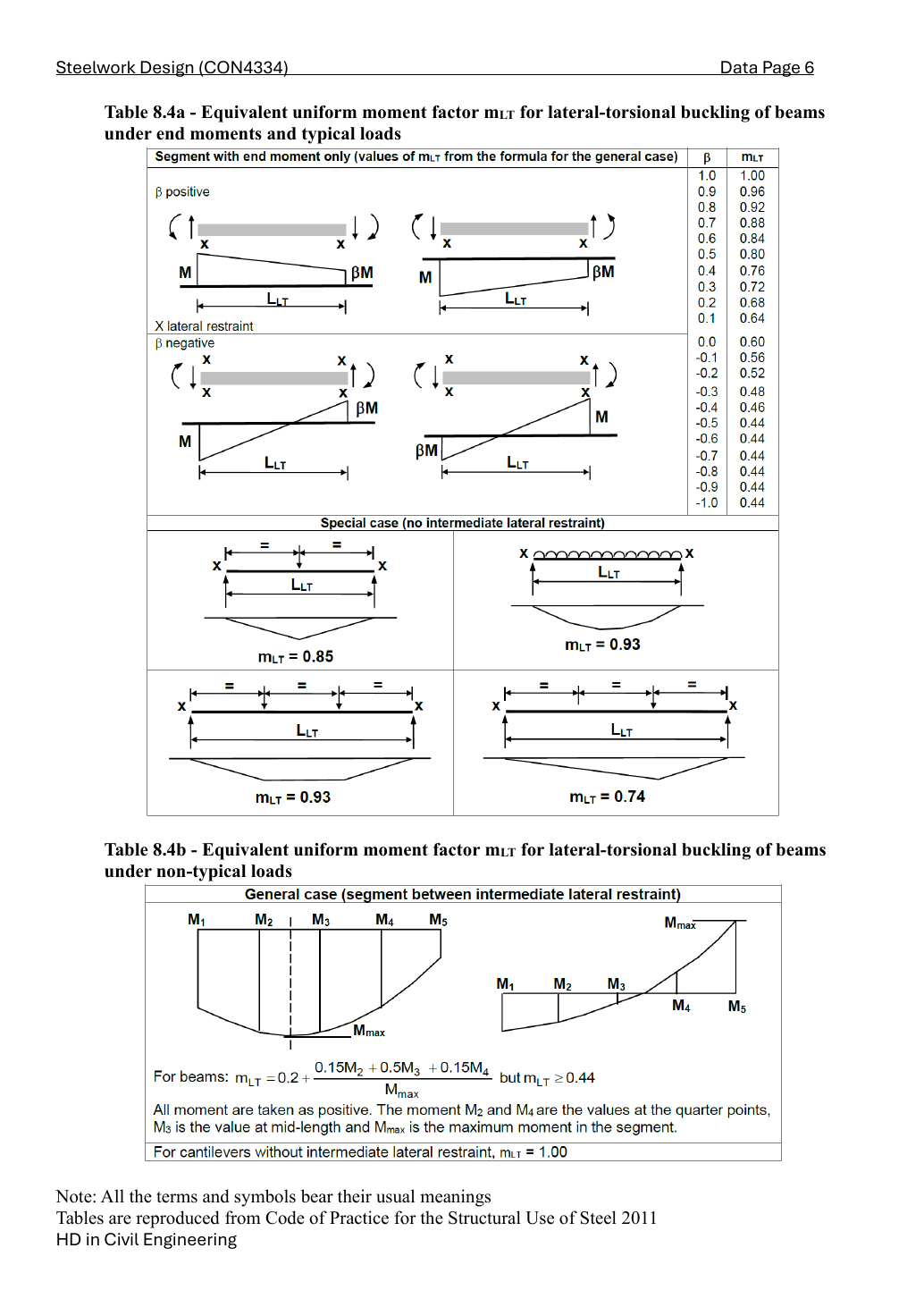
Table 8.4a: equivalent uniform moment factor for beam LTB under end moments and standard loading cases, . X denotes lateral restraint; is the segment length between two restraints; the end moments are and . For the upper straight-line moment diagram with one sign, is positive. For the lower diagram crossing zero, is negative. Do not decide the signs of internal moments solely from applied arrow directions.
| — | — |
All four special-case diagrams have no intermediate lateral restraint: one midspan point load ; full-span UDL ; two loads at the third points ; one load at a third point . Equality marks denote equal segment lengths. Arrows are the loads/reactions shown; do not scale unlabelled dimensions from the drawing.
Table 8.4b: for a general segment under nonstandard loading, use segment ends , , quarter points , , midpoint and segment maximum . Use positive magnitudes throughout; , but . For a cantilever without intermediate lateral restraint, .
Animation labRead the moment shape within one segment
Supplement to the original lesson. Enable JavaScript to play, step through calculations and rotate 3D models. The following explanation remains readable offline.
- Moment ordinates must belong to the same effective unbraced segment.
- Same-side and reverse-curvature diagrams have different signed end ratios.
- The markers show ¼, ½ and ¾ of this segment, not of the entire beam.
- LTB and column flexural factors are different. Preserve their individual bounds and coefficient sets.
Data File 7: Tables 8.7 and 8.9: curves and flexural moment
First select the buckling curve by section type, thickness and axis. For a hot-rolled H-section with thickness , about the axis use b; about the axis use c. Then select the flexural-buckling moment factor from the relevant moment diagram; it need not equal the LTB factor. For a straight-line end-moment diagram, when , ; when , . Establish the internal-moment signs from the external arrow convention in the question. Ordinary flexural-buckling quarter-point ordinates retain their signs, unlike LTB.
Full method and worked application.
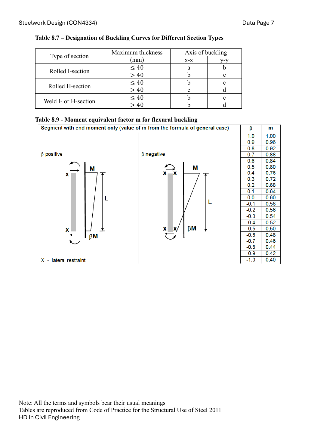
| Section | Maximum thickness () | About | About |
|---|---|---|---|
| Hot-rolled I-section | a | b | |
| Hot-rolled I-section | b | c | |
| Hot-rolled H-section | b | c | |
| Hot-rolled H-section | c | d | |
| Welded I/H-section | b | c | |
| Welded I/H-section | b | d |
Table 8.9: equivalent moment factor for flexural buckling in a segment subject only to end moments. X denotes lateral restraint; is segment length; internal end moments are , . The left diagram has same-sign moments and is positive; the right diagram has opposite-sign moments and is negative. Values follow below. Do not substitute the negative-ratio portion of Table 8.4a.
| — | — |
Animation labEffective length and buckling axes
Supplement to the original lesson. Enable JavaScript to play, step through calculations and rotate 3D models. The following explanation remains readable offline.
- A column can bow sideways before its section reaches the crushing resistance.
- Each axis has its own radius of gyration and restraint spacing.
- , with compatible length units. A tie affects only the directions it actually restrains.
- Select each buckling curve and compressive strength before forming Pc. The governing axis is determined by resistance, not slenderness alone.
Data File 8: Table 8.8: compression strength
Use three keys: curve, material design strength and . If curve c, and , rows / give /; . With , . Repeat for the other axis and retain the governing resistance. Data File curve b, py 355, λ90 prints “”; the full lecture Ch 4 p 8 clearly gives , which this site uses.
Full method and worked application.
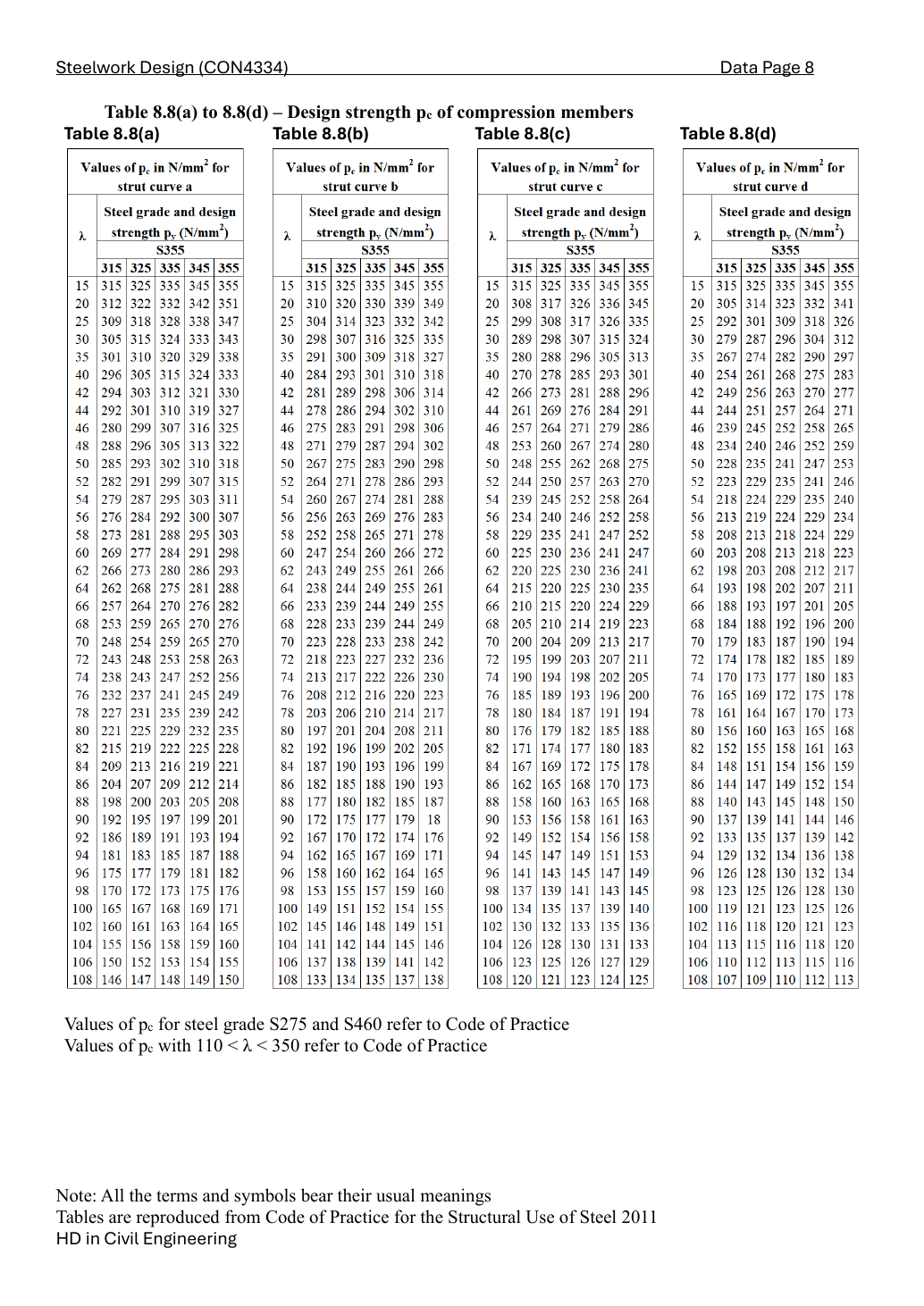
Tables 8.8(a), (b), (c) and (d) give , in for strut curves a, b, c and d respectively. Rows in each table give ; this page lists only S355. The printed columns are, in order, . rows must be selected as shown; their spacing is not uniform throughout. The source directs the reader to the code for S275, S460 and of . Do not fill in unprinted values. For curve b in the , column, the source value differs from the complete lecture; see the explicit source correction above. The HTML below extracts the curve b/c / columns; has the same units as above.
| b / py 345 | b / py 355 | c / py 345 | c / py 355 | |
|---|---|---|---|---|
Animation labEffective length and buckling axes
Supplement to the original lesson. Enable JavaScript to play, step through calculations and rotate 3D models. The following explanation remains readable offline.
- A column can bow sideways before its section reaches the crushing resistance.
- Each axis has its own radius of gyration and restraint spacing.
- , with compatible length units. A tie affects only the directions it actually restrains.
- Select each buckling curve and compressive strength before forming Pc. The governing axis is determined by resistance, not slenderness alone.
Data File 9: UB dimensions: identify the exact row
Match all three designation numbers, including mass. Read actual depth , width , web , flange , root radius , clear web depth and tabulated ,. The nominal name does not mean its exact depth is or its web is thick. Dimension-table is not bolt diameter; its meaning changes with context. A larger flange thickness can lower and must be checked after selection.
Full method and worked application.
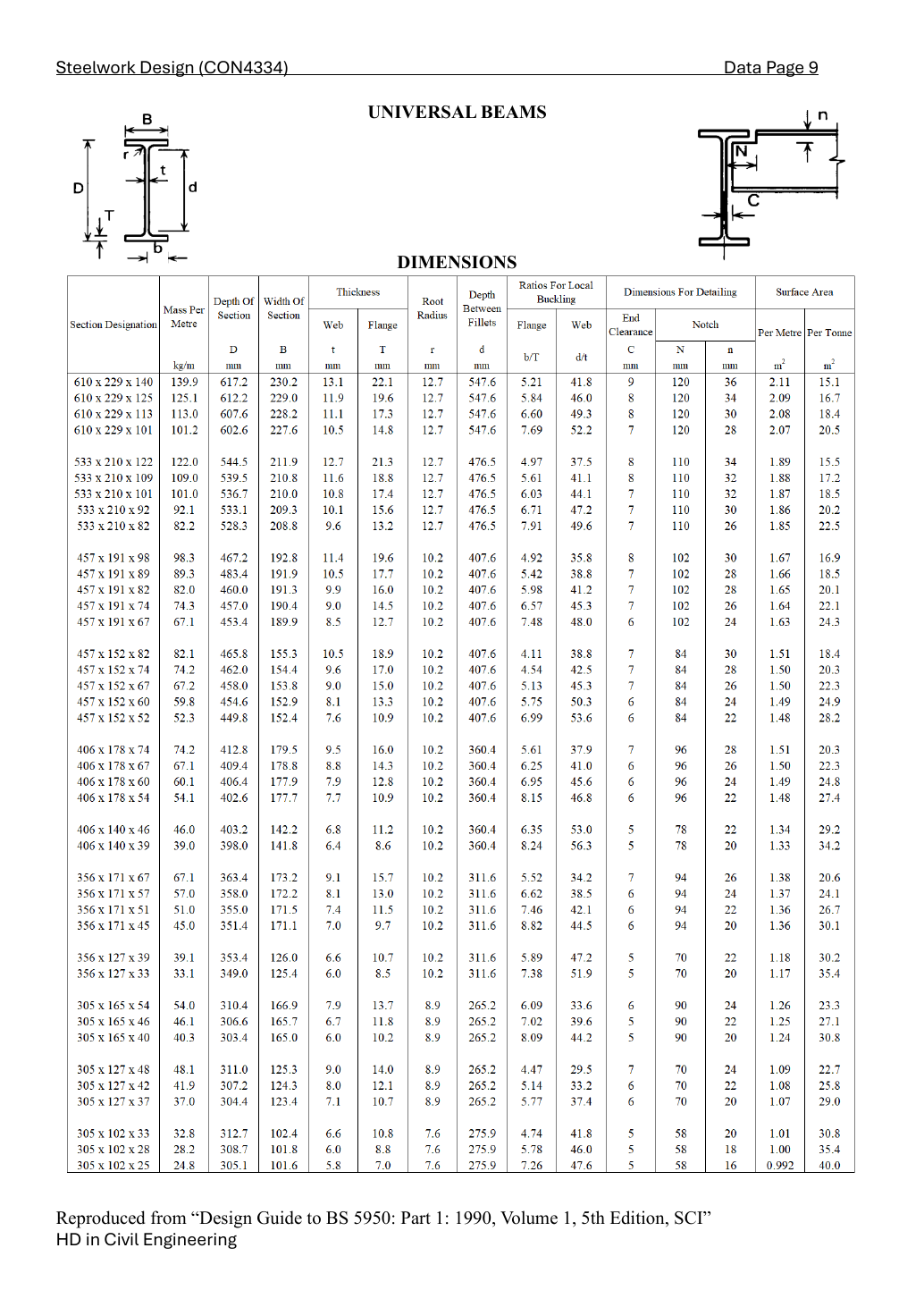
UNIVERSAL BEAMS / DIMENSIONS. In the upper-left section sketch, spans overall section depth; spans full flange width; crosses web thickness; crosses flange thickness; points to the root fillet; spans clear web depth between root fillets; is the flange outstand width shown. Classification still uses the tabulated ratios. In the upper-right notch sketch, is end clearance; is horizontal notch dimension; is vertical notch dimension. This is not the question's load diagram and specifies no actual beam length.
Column headings: Section Designation; Mass Per Metre, ; Depth / Width / Web / Flange / Root Radius / Depth Between Fillets correspond respectively to , , , , , , all in ; Ratios for Local Buckling give flange and web , both dimensionless; Dimensions for Detailing, , , uses . Finally, the two Surface Area columns are per metre and per tonne, in . The source page credits Design Guide to BS 5950: Part 1: 1990, Volume 1, 5th Edition, SCI as the publication source of the supplied section tables. The design method still follows the course Hong Kong code.
Animation labExplore section geometry and axes
Supplement to the original lesson. Enable JavaScript to play, step through calculations and rotate 3D models. The following explanation remains readable offline.
- The flanges are the wide plates; the web connects them. Rotate the I-section to see both.
- The same section has different stiffness and resistance about its two principal axes.
- I controls elastic curvature; is elastic section modulus. Plastic modulus S comes from plastic stress blocks.
- Nominal section labels are not every actual dimension. Keep the row, axis and units together.
Data File 10: UB properties: keep axes and units
Use the same complete section designation as the dimension table. Read , in (×→), , in (×→), , and , in (×→), area in (×→), plus dimensionless and torsional index . Use for major-axis vertical deflection, for LTB slenderness, for Class 1/2 bending and elastic for the specified column member equations. Never interpolate between different section sizes to create a fictional section.
Full method and worked application.
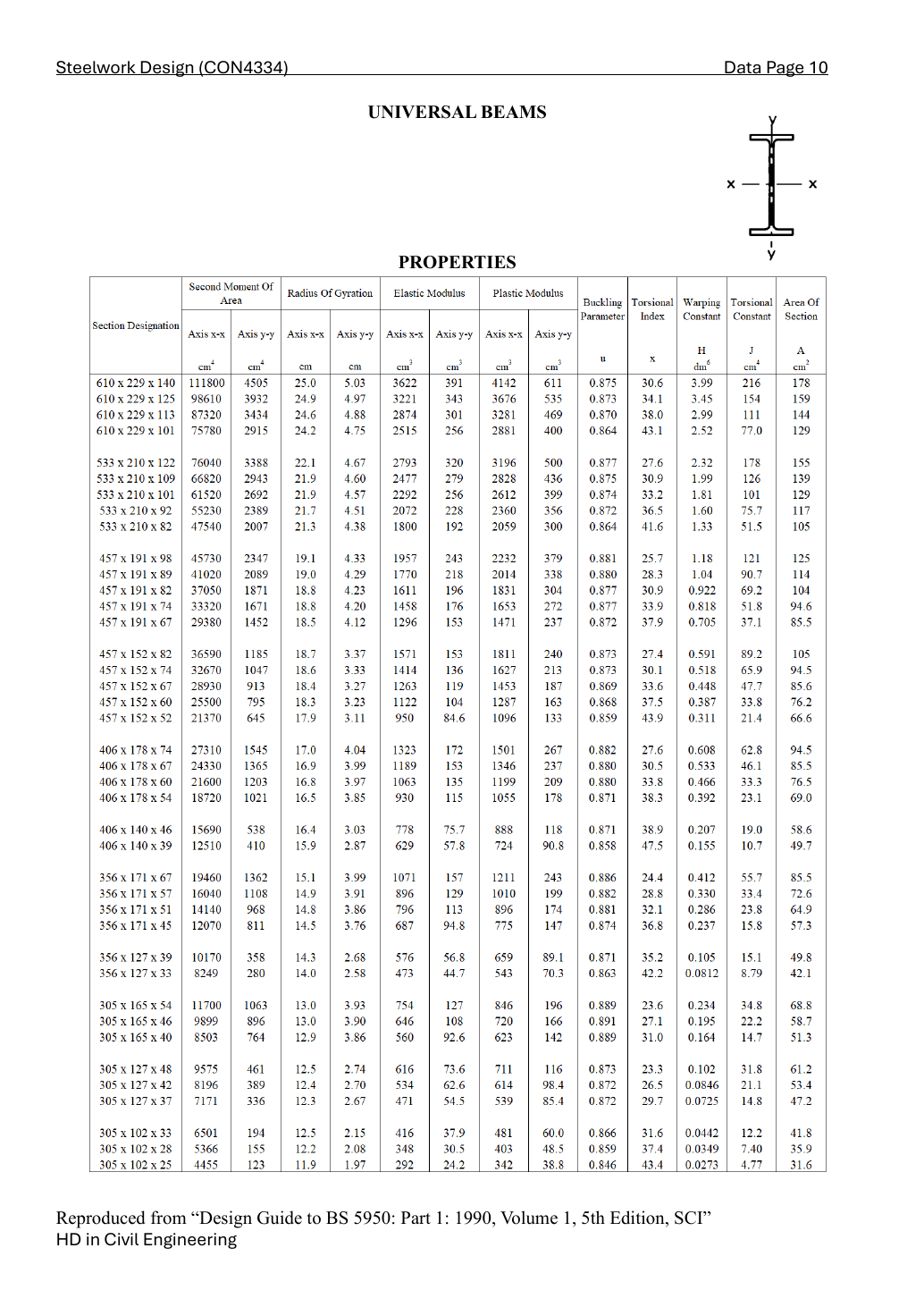
UNIVERSAL BEAMS / PROPERTIES. In the upper-right sketch, horizontal is the major axis and vertical is the minor axis, both through the centroid. No applied load is shown. Columns give Second Moment of Area, in order , (); Radius of Gyration, , (); Elastic Modulus, , (); Plastic Modulus, , (). Here Modulus means section modulus, not the material's Young's modulus.
Buckling Parameter ; Torsional Index , not the axis; Warping Constant (source table ); Torsional Constant (); Area of Section (). This is the section's torsional constant, not the line-weld group polar inertia . The source page is extracted from Design Guide to BS 5950: Part 1: 1990, Volume 1, 5th Edition, SCI; all selected properties must belong to the same section row.
Animation labExplore section geometry and axes
Supplement to the original lesson. Enable JavaScript to play, step through calculations and rotate 3D models. The following explanation remains readable offline.
- The flanges are the wide plates; the web connects them. Rotate the I-section to see both.
- The same section has different stiffness and resistance about its two principal axes.
- I controls elastic curvature; is elastic section modulus. Plastic modulus S comes from plastic stress blocks.
- Nominal section labels are not every actual dimension. Keep the row, axis and units together.
Data File 11: UC dimensions and properties
The separate data file places UC dimensions and properties together. Read along exactly the same section row, then use the rough check is consistent with mass per metre. This only screens for transcription mistakes and does not replace tabulated values. The larger UC needed for Assignment 2 is absent from this page but is supplied in 2023 Data pp.16–17. That solution explicitly cites its lookup source.
Full method and worked application.
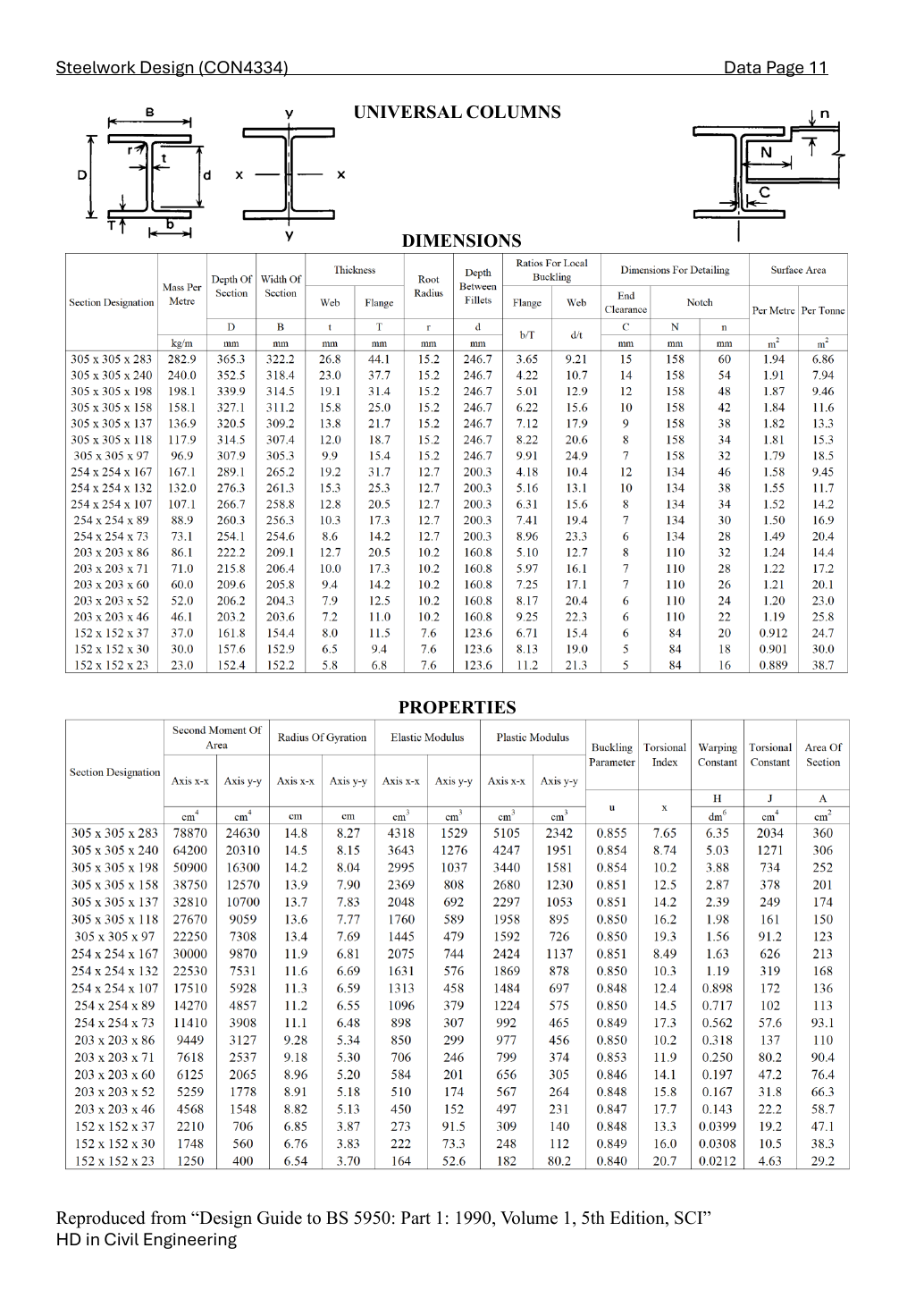
UNIVERSAL COLUMNS. In the upper-left dimension sketch, is overall depth; full width; web thickness; flange thickness; root radius; clear web depth between fillets; the flange outstand shown. In the upper-middle axes sketch, horizontal is the major axis and vertical the minor axis. In the upper-right joint sketch, , , are end clearance, horizontal notch dimension and vertical notch dimension respectively, not column height or restraint spacing.
Upper DIMENSIONS table: mass per metre is in ; , , , , , , , , uses ; local-buckling ratios , are dimensionless; the last two columns give surface area per metre/per tonne in . Lower PROPERTIES table: second moment , (), radius of gyration , (), elastic section modulus , and plastic section modulus , (), buckling parameter , torsional index , warping constant (), torsional constant (), area (). The upper and lower tables must match the same complete section designation. Source publication: Design Guide to BS 5950: Part 1: 1990, Volume 1, 5th Edition, SCI.
Animation labExplore section geometry and axes
Supplement to the original lesson. Enable JavaScript to play, step through calculations and rotate 3D models. The following explanation remains readable offline.
- The flanges are the wide plates; the web connects them. Rotate the I-section to see both.
- The same section has different stiffness and resistance about its two principal axes.
- I controls elastic curvature; is elastic section modulus. Plastic modulus S comes from plastic stress blocks.
- Nominal section labels are not every actual dimension. Keep the row, axis and units together.
Data File 12: Unequal angles: orient the centroid
Match long leg, short leg and thickness; read the small axis sketch before selecting or . For an angle whose long leg is connected, the distance from heel to centroid along that leg determines balanced longitudinal weld forces. This is not generally half the leg length. The table includes rolled root effects; simple rectangular angle areas in worked questions are identified as that course approximation. The standalone block contains inconsistent thickness labels; do not borrow an uncertain area for the question.
Full method and worked application.
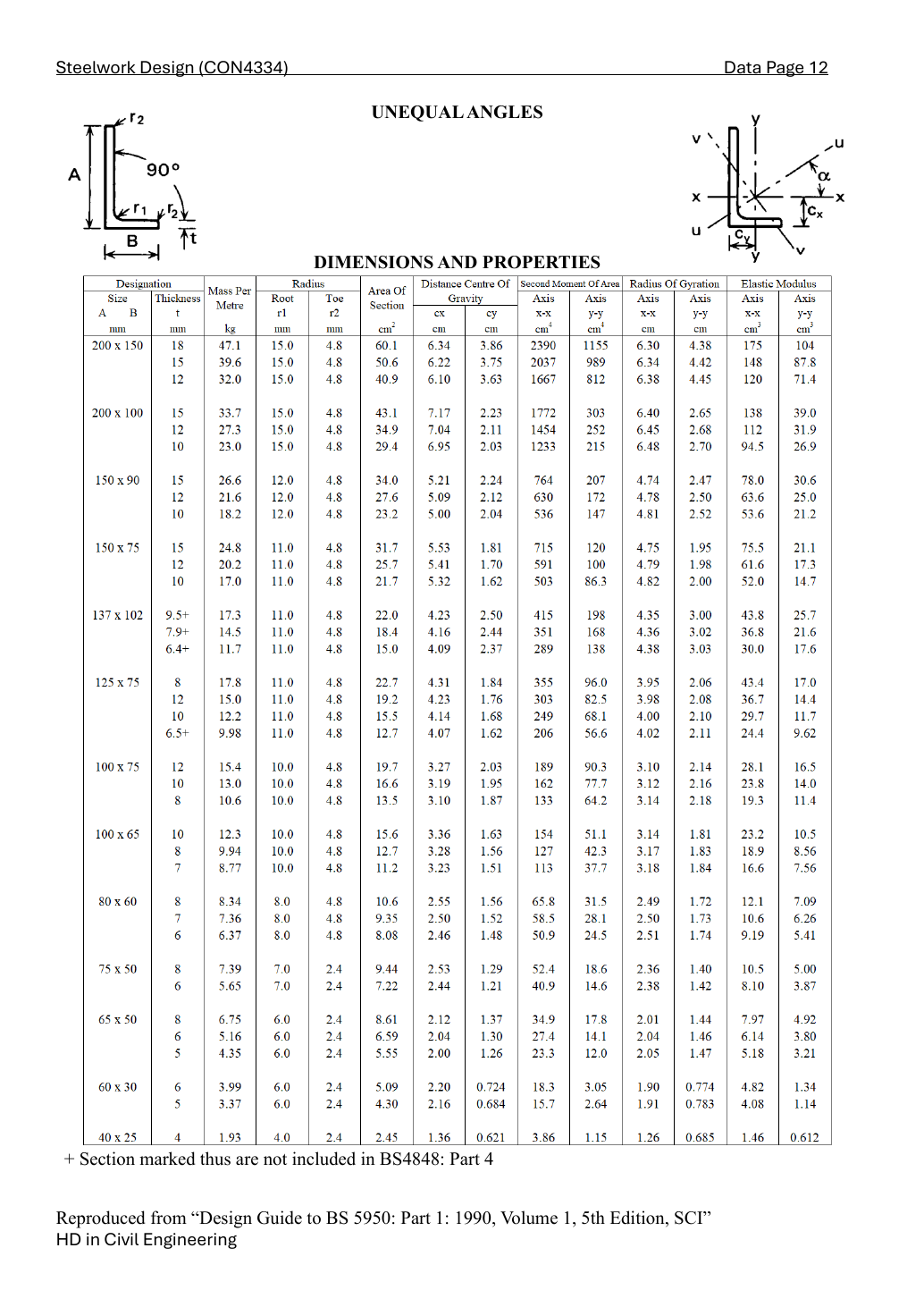
UNEQUAL ANGLES / DIMENSIONS AND PROPERTIES. Upper-left sketch: is the full vertical long-leg length; the full horizontal short-leg length; leg thickness; included angle , is the internal root radius; is the toe radius. Upper-right sketch: is horizontal; is vertical; they intersect at the centroid. is the vertical distance from the short leg's outer back to the horizontal centroidal axis; is the horizontal distance from the long leg's outer back to the vertical centroidal axis. Inclined axes , are the principal axes; is their shown rotation. A subscript does not make a horizontally measured distance.
Column order: dimensions , and thickness (); mass per metre (the source heading prints ; “per metre” is stated in Mass Per Metre); root and toe (); section area (); centroid distances , (); about , , second moment (), radius of gyration (), elastic section modulus (). A + after the thickness is a source note: that section is not included in BS4848: Part 4. It does not mean addition of dimensions.: the first three row thickness labels print, in order, , but mass/area ordering is inconsistent. Retain the source image and apply the limitations explained above. Source publication: Design Guide to BS 5950: Part 1: 1990, Volume 1, 5th Edition, SCI.
Animation labBalance two weld forces
Supplement to the original lesson. Enable JavaScript to play, step through calculations and rotate 3D models. The following explanation remains readable offline.
- The angle centroid/load line is generally not halfway between the two weld runs.
- . Both weld runs contribute to the applied force.
- . The run nearer the load line carries more force.
- For equal throat resistance per length, the required effective lengths follow the same ratio. Add detailing allowances afterwards.
2023 attachment 1: Beam, tension and elastic properties
This is printed Data page 1, physical PDF page 7, in Pastpaper/22ENGTY033.pdf. Class 1/2 low-shear ; . Simply supported deflection: full-span UDL ; central point load . For LTB use , then compare . Angle tension uses the appropriate bolted/welded, single/double reduction of outstanding-leg area . Compression uses , with read for each axis. The point-load exponent printed on this Data File page is : this is dimensionally wrong; the lecture, Word note and 2023 data show . The central-point-load formula on THIS examination sheet correctly uses .
Detailed lookup rules and units.
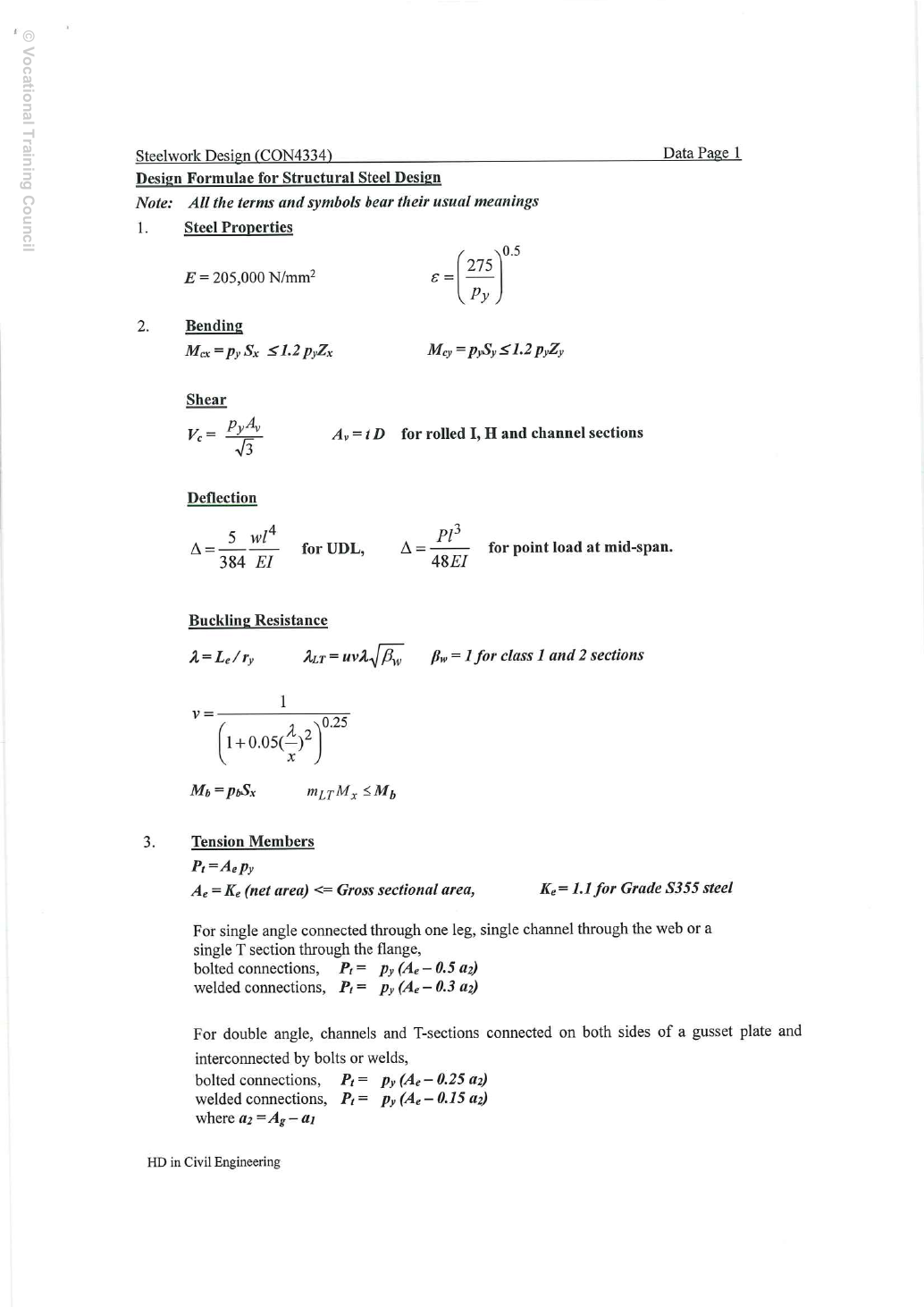
Source headings: Steelwork Design (CON4334); Design Formulae for Structural Steel Design. Symbols are stated to have their usual meanings. Item 1, steel properties: ,.
Item 2, bending: ,; applicable section classes and low-shear conditions are explained above. Shear: ; for hot-rolled I, H and channel sections, use . Deflection under a full-span UDL: ; midspan point load . This source uses lower-case span ; its point-load formula does have the correct cubic power.
Buckling resistance: ,; for Classes 1/2, ; ; ,. is section torsional index, not a position coordinate.
Item 3, tension members: ,; for S355, . Single angle connected through one leg, single channel through its web or single tee through its flange: bolted ; welded: . Paired angles/channels/tees on opposite gusset faces and interconnected by bolts or welds: bolted ; welded: ; . The footer identifies HD in Civil Engineering; the side carries the Vocational Training Council copyright notice.
Animation labCompression and tension across a section
Supplement to the original lesson. Enable JavaScript to play, step through calculations and rotate 3D models. The following explanation remains readable offline.
- For sagging, the top flange is in compression and the bottom in tension; hogging reverses this.
- Elastic bending stress varies with distance from the neutral axis: .
- The section class governs whether elastic, plastic or effective properties may be used.
- Use the shear at the section under examination; the largest shear elsewhere is not automatically coexistent.
2023 attachment 2: Compression, column checks and bolt bearing
This is printed Data page 2, physical PDF page 8, in Pastpaper/22ENGTY033.pdf. The compact column equations omit information visible in the full lecture, including elastic denominators and amplified-moment notation. Use the linked column method to restore these details. For a rectangular four-sided line weld of width and height : , , and , all line inertias in . At coordinates , torsional components are and in when is . Add direct components before taking the resultant. These formulas do not describe a missing-side weld.
Detailed lookup rules and units.
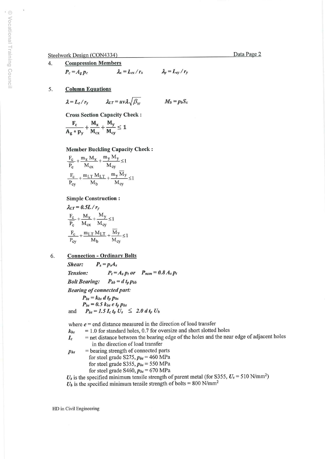
Item 4, compression members: ,,. Item 5, columns: ,,.
Section check: . Member buckling expressions as printed: ; .
Original simple-construction expression: ; ; . The final source expression retains and is not identical to the separate Data File shorthand. Original overbars and denominators are retained here. In a solution, use the full lecture definitions of elastic moment resistance, amplified moments and simple-construction factors; the summary table is not a complete definition.
Item 6, ordinary bolts: ; ; the specified interaction expression instead uses ; bolt bearing . Original connected-part bearing expressions, in order: , , and ; these are limits, not resistances to add.
is end distance along the load-transfer direction. Standard holes: ; oversized and short-slotted holes: ; is the clear distance along load transfer from the hole's bearing edge to the nearest edge of the next hole. Connected-part bearing strength: S275 ,S355 ,S460 . Parent-metal minimum tensile strength ; for S355, use . The page gives bolt for the course Grade 8.8 cases, not every grade. The footer identifies HD in Civil Engineering.
Animation labEffective length and buckling axes
Supplement to the original lesson. Enable JavaScript to play, step through calculations and rotate 3D models. The following explanation remains readable offline.
- A column can bow sideways before its section reaches the crushing resistance.
- Each axis has its own radius of gyration and restraint spacing.
- , with compatible length units. A tie affects only the directions it actually restrains.
- Select each buckling curve and compressive strength before forming Pc. The governing axis is determined by resistance, not slenderness alone.
2023 attachment 3: Eccentric fasteners, weld strength and bolt areas
This is printed Data page 3, physical PDF page 9, in Pastpaper/22ENGTY033.pdf. Choose the nominal diameter row; use tensile area for tension and thread shear, shank area only for an unthreaded shear plane. Grade selects ,,. For double shear count two planes, but bearing depends on the actual contacting plate thickness. Check connected-part bearing with the diameter term, end-distance term and clear-ligament/bolt-tensile cap. For eccentric groups use the correct centroid or rotation pivot. The combined shear/tension limit is plus individual checks, not a replacement for them.
Detailed lookup rules and units.
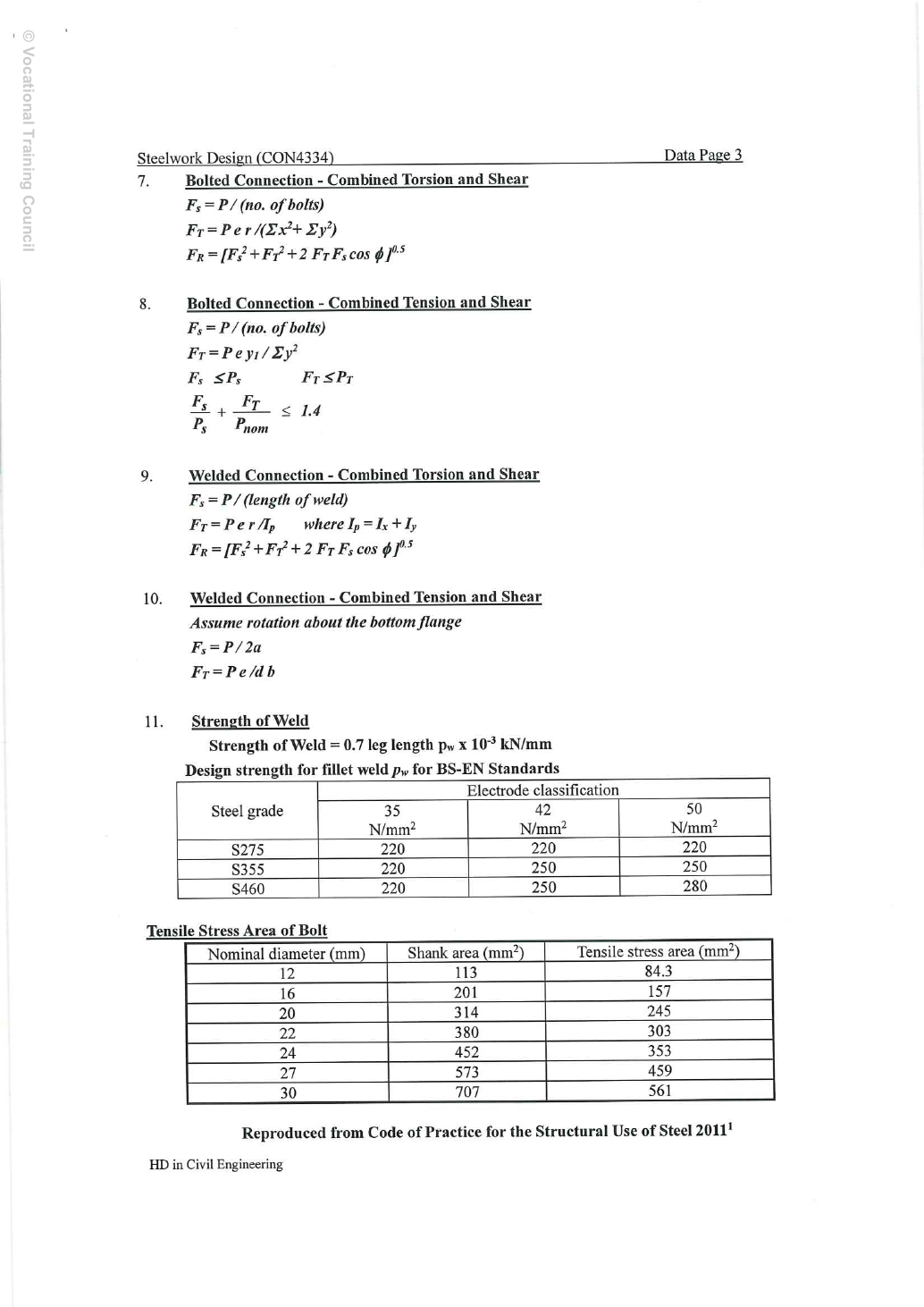
Item 7, bolt torsion and shear: ,,. Item 8, bolt tension and shear: ,,,,. The tension limit uses an upper-case subscript ; the preceding page defines . Recognise their correspondence in the same tension check.
Item 9, weld torsion and shear: ,,,. Item 10, weld tension and shear, assuming rotation about the bottom flange: ,. This exam expression uses lower-case , , while the separate Data File uses upper-case dimensions. There is no geometry sketch on this page; confirm measurement locations from the actual question instead of assuming identical section symbols. The torsion expressions' and the tension expressions' have different physical meanings.
Item 11, weld strength: ; leg length is the weld leg entered in millimetres; uses . Both tables below have been compared cell by cell with this image; electrode designations are not strength values.
| Steel grade | 35 | 42 | 50 |
|---|---|---|---|
| S275 | |||
| S355 | |||
| S460 |
| Nominal diameter () | Shank area () | Tensile stress area () |
|---|---|---|
The page credits the Hong Kong 2011 steel code. In the bolt table, tensile stress area applies to tension/threaded shear; shank area applies only to the corresponding unthreaded shear plane.
Animation labAdd direct and torsional bolt forces
Supplement to the original lesson. Enable JavaScript to play, step through calculations and rotate 3D models. The following explanation remains readable offline.
- Assign signed coordinates to the bolts relative to the group centroid.
- For the equal-bolt elastic model, the direct force is per bolt.
- Moment magnitude is ; its sign follows the load direction. For signed M: , , .
- Add signed x and y components at each bolt, then take the resultant. The longest arrow shows the critical bolt in this illustration.
2023 attachment 4: Bolt strengths, steel strengths, section class and SLS limits
This is printed Data page 4, physical PDF page 10, in Pastpaper/22ENGTY033.pdf. Read the steel-grade heading, then the first thickness upper bound that contains the actual governing thickness. For S355, uses ; uses the row, . Calculate . In Table 7.1 select flange/web, rolled/welded and bending/compression stress pattern; compare and to the class limits. Take the worse element class. The compression stress parameter is bounded between and ; do not use a pure-bending web limit for uniform compression.
Detailed lookup rules and units.
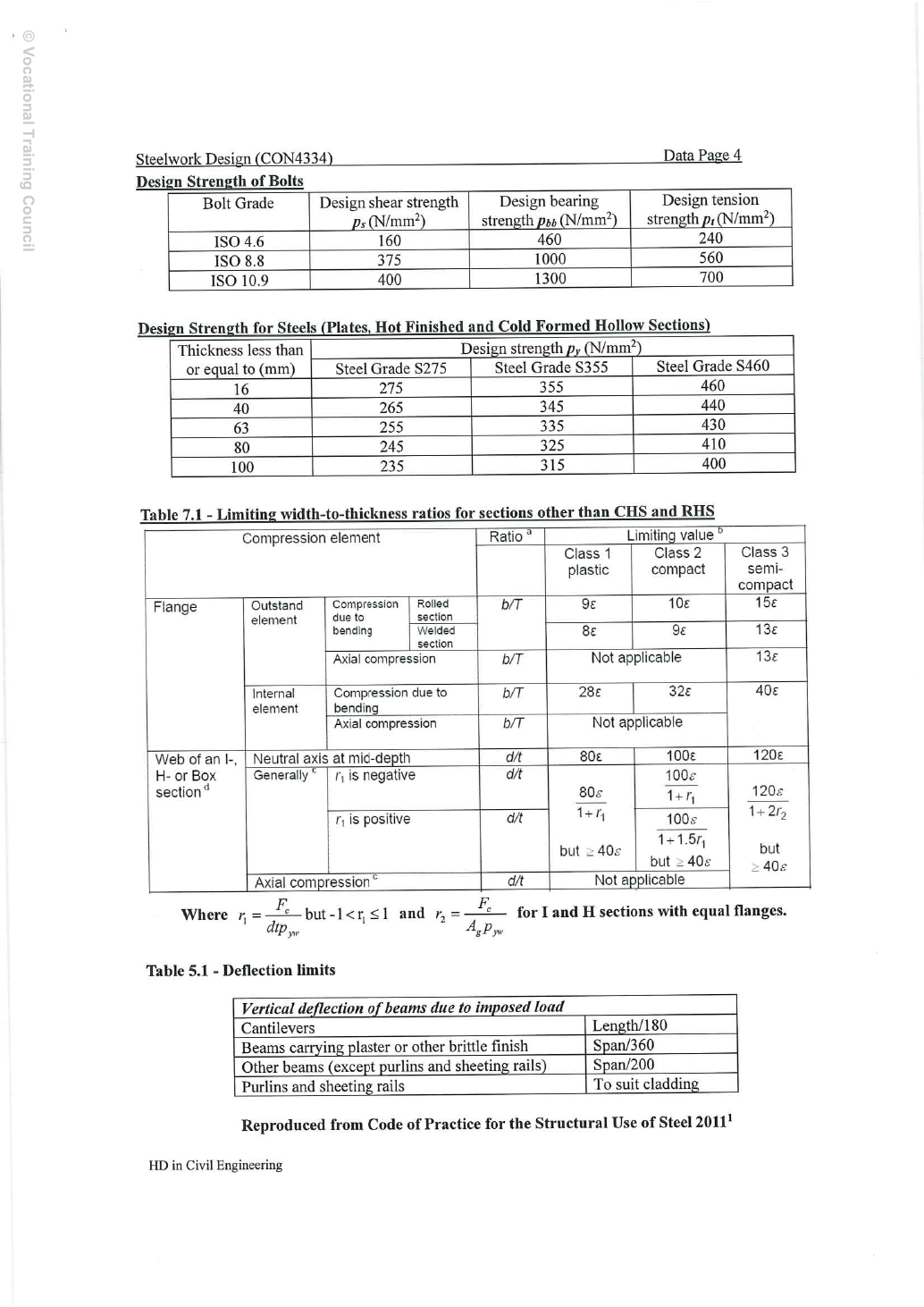
The tables below match this image's bolt strengths, material thickness/strength and classification cell by cell. The material table heading covers plates and hot-finished/cold-formed hollow sections. Formula symbols are unchanged; merged cells are restated for their applicable rows.
| Bolt grade | Shear | Bearing | Tension |
|---|---|---|---|
| ISO 4.6 | |||
| ISO 8.8 | |||
| ISO 10.9 |
| Upper thickness limit () | S275 | S355 | S460 |
|---|---|---|---|
| Compression element / stress pattern | Ratio | Class 1 | Class 2 | Class 3 |
|---|---|---|---|---|
| Hot-rolled flange outstand in compression from bending | ||||
| Welded flange outstand in compression from bending | ||||
| Flange outstand under axial compression | Not applicable | Not applicable | ||
| Internal flange element in compression from bending | ||||
| Internal flange element under axial compression | Not applicable | Not applicable | ||
| I/H/box web with neutral axis at mid-depth | ||||
| General web case, negative | ; the source notes | , and | ||
| General web case, positive | ; the source notes | , and | , and | |
| Web under axial compression | Not applicable | Not applicable | , and |
Original expression below the table ; here the source prints ; for equal-flange I/H-sections, . In this appendix the Class 1 lower boundary prints , unlike the separate Data File's . Both source forms are retained, without silently making them identical. General lookup teaching above still requires the full course definitions; in particular, makes the denominator zero and cannot be substituted directly.
Table 5.1, vertical deflection due to imposed load: cantilever limit ; beams supporting plaster/other brittle finishes ; other beams excluding purlins and sheeting rails ; purlins and sheeting rails follow cladding requirements. The page credits the Hong Kong 2011 steel code.
Animation labRead a table without losing the keys
Supplement to the original lesson. Enable JavaScript to play, step through calculations and rotate 3D models. The following explanation remains readable offline.
- Name the required property: material strength, section property, buckling strength or a moment factor.
- Keep section size, steel grade, thickness band, curve and axis as separate lookup keys.
- , and require different conversion powers. Do not use adjacent columns interchangeably.
- Use bracketing rows within the same valid column. The original page remains the source of all table values.
2023 attachment 5: LTB strength table
This is printed Data page 5, physical PDF page 11, in Pastpaper/22ENGTY033.pdf. First calculate , not merely . Choose the column within the steel grade. Locate its two surrounding rows, interpolate linearly and multiply by . If the input exceeds available rows, obtain the applicable source table rather than extrapolating. For a value below the first printed row , this site conservatively uses row ; it never makes exceed . at the bottom indicates the negligible-buckling range and is not an extra multiplier.
Detailed lookup rules and units.
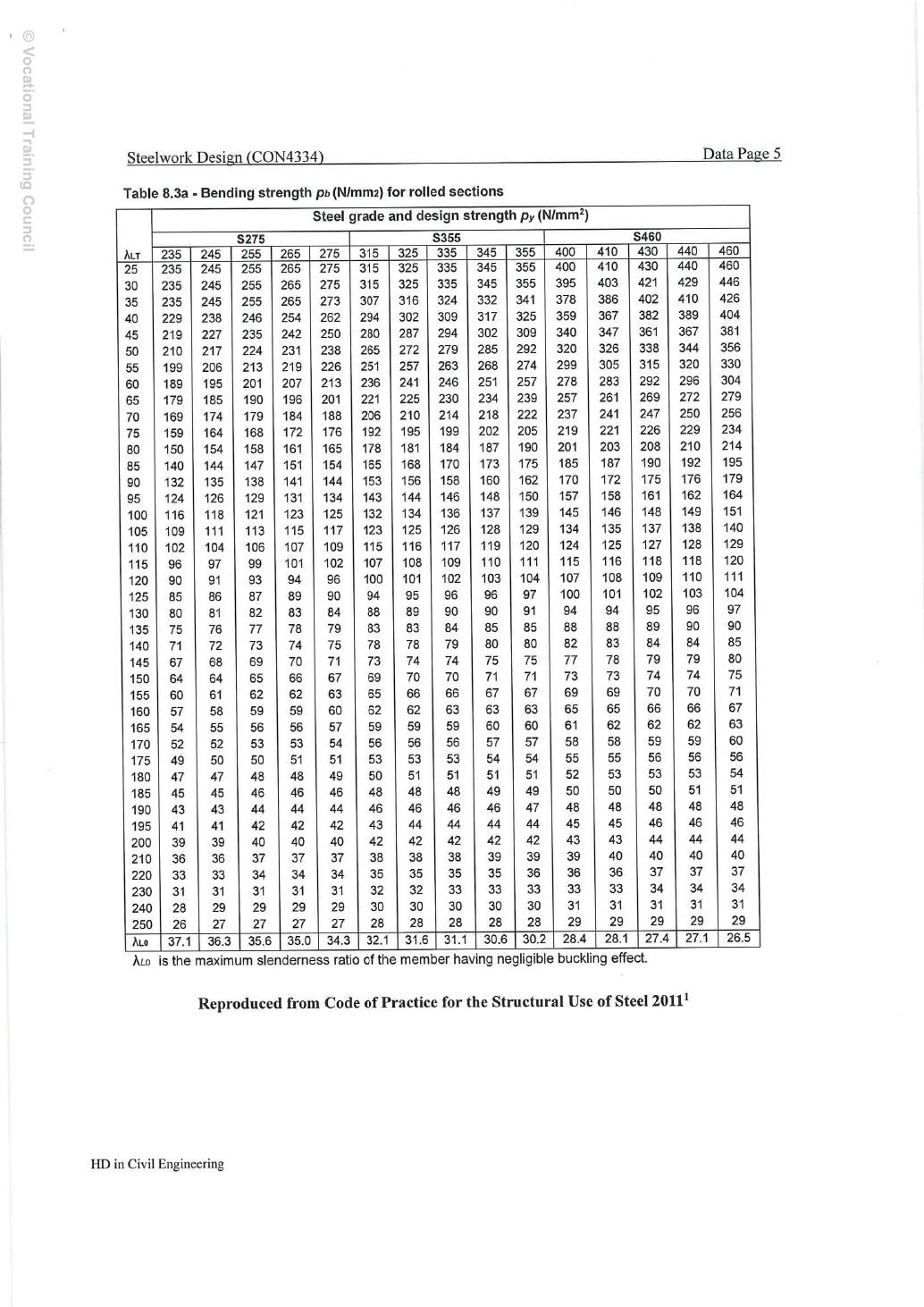
Source heading: bending strength of hot-rolled sections , in ; rows give . For S275, the columns are, in order, ; for S355, ; for S460, , with the same units. The bottom row gives the maximum slenderness at which member-buckling effects can be neglected. In the same column order, S275: ; S355: ; S460: .
This exam table also uses the steel-grade/design-strength column and row to look up . Source column lines confirm that the 355 column at rows gives ; the adjacent 400-column values do not belong to that column. At rows , the 355-column values are respectively . The four old HTML transcription differences are explicitly listed in the Data File 5 legend. The table footer defines as maximum slenderness at which buckling effects can be neglected, not a multiplier. The page credits the Hong Kong 2011 steel code.
Animation labA beam bends sideways and twists
Supplement to the original lesson. Enable JavaScript to play, step through calculations and rotate 3D models. The following explanation remains readable offline.
- For the illustrated sagging beam the top flange is compressed.
- The unrestrained compression flange can move sideways while the complete cross-section twists.
- Only effective restraints divide the member into unbraced segments. They do not automatically add vertical supports.
- Use the segment effective length, section properties and matching moment factor. This is an exaggerated mode shape, not a calculated displacement.
2023 attachment 6: LTB moment factors
This is printed Data page 6, physical PDF page 12, in Pastpaper/22ENGTY033.pdf. Match the whole unrestrained segment to the sketch, including its end moments and intermediate loads. A simply supported central point load uses ; a full-span UDL uses the supplied shortcut. For a general diagram use the absolute quarter-point ordinates in Table 8.4b and its minimum . If a more accurate quarter-point result differs slightly from a shortcut, state which prescribed method you used. Cantilevers without intermediate restraint use under the supplied table.
Detailed lookup rules and units.
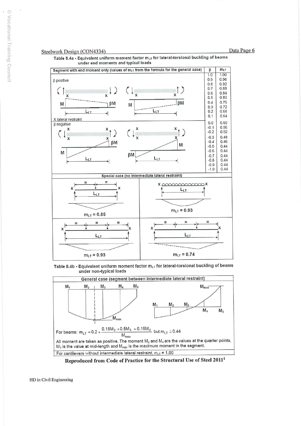
Table 8.4a: equivalent uniform moment factor for beam LTB under end moments and standard loading cases, . X denotes lateral restraint; is the segment length between two restraints; the end moments are and . For the upper straight-line moment diagram with one sign, is positive. For the lower diagram crossing zero, is negative. Do not decide the signs of internal moments solely from applied arrow directions.
| — | — |
All four special-case diagrams have no intermediate lateral restraint: one midspan point load ; full-span UDL ; two loads at the third points ; one load at a third point . Equality marks denote equal segment lengths. Arrows are the loads/reactions shown; do not scale unlabelled dimensions from the drawing.
Table 8.4b: for a general segment under nonstandard loading, use segment ends , , quarter points , , midpoint and segment maximum . Use positive magnitudes throughout; , but . For a cantilever without intermediate lateral restraint, .
The factors, formulas and diagram labels above have been compared individually with this exam image. The page credits the Hong Kong 2011 steel code.
Animation labRead the moment shape within one segment
Supplement to the original lesson. Enable JavaScript to play, step through calculations and rotate 3D models. The following explanation remains readable offline.
- Moment ordinates must belong to the same effective unbraced segment.
- Same-side and reverse-curvature diagrams have different signed end ratios.
- The markers show ¼, ½ and ¾ of this segment, not of the entire beam.
- LTB and column flexural factors are different. Preserve their individual bounds and coefficient sets.
2023 attachment 7: Flexural moment factors and strut curve selection
Source: Pastpaper/22ENGTY033.pdf, printed Data p.7, physical PDF p.13. First select the buckling curve by section type, thickness and axis. For a hot-rolled H-section with thickness , about the axis use b; about the axis use c. Then select the flexural-buckling moment factor from the relevant moment diagram; it need not equal the LTB factor. For a straight-line end-moment diagram, when , ; when , . Establish the internal-moment signs from the external arrow convention in the question. Ordinary flexural-buckling quarter-point ordinates retain their signs, unlike LTB.
Detailed lookup rules and units.
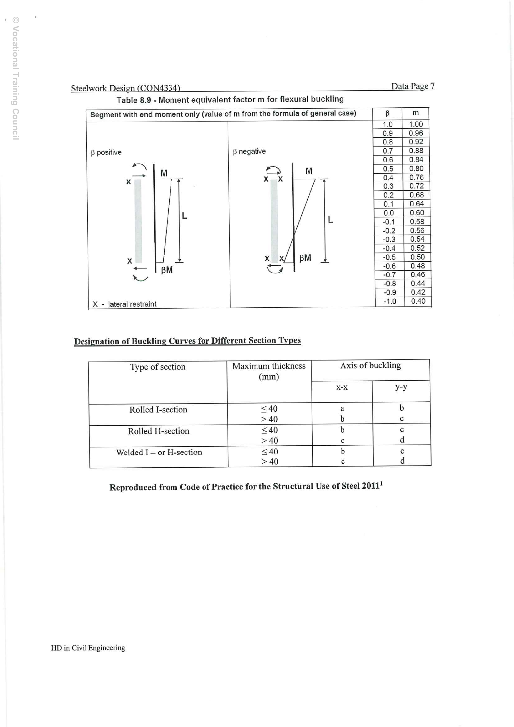
| Section | Maximum thickness () | About | About |
|---|---|---|---|
| Hot-rolled I-section | a | b | |
| Hot-rolled I-section | b | c | |
| Hot-rolled H-section | b | c | |
| Hot-rolled H-section | c | d | |
| Welded I/H-section | b | c | |
| Welded I/H-section | c | d |
Table 8.9: equivalent moment factor for flexural buckling in a segment subject only to end moments. X denotes lateral restraint; is segment length; internal end moments are , . The left diagram has same-sign moments and is positive; the right diagram has opposite-sign moments and is negative. Values follow below. Do not substitute the negative-ratio portion of Table 8.4a.
| — | — |
Source discrepancy: In the lower curve table of this paper, the welded I/H-section row at thickness and about prints c; the corresponding cell on separate Data File p.7 prints b. This transcription retains the exam's c. The tables are not identical; if a question uses this case, explicitly identify the chosen source. The page credits the Hong Kong 2011 steel code.
Animation labRead the moment shape within one segment
Supplement to the original lesson. Enable JavaScript to play, step through calculations and rotate 3D models. The following explanation remains readable offline.
- Moment ordinates must belong to the same effective unbraced segment.
- Same-side and reverse-curvature diagrams have different signed end ratios.
- The markers show ¼, ½ and ¾ of this segment, not of the entire beam.
- LTB and column flexural factors are different. Preserve their individual bounds and coefficient sets.
2023 attachment 8: Compression curve a
This is printed Data page 8, physical PDF page 14, in Pastpaper/22ENGTY033.pdf. Use three keys: curve, material design strength and . If curve c, and , rows / give /; . With , . Repeat for the other axis and retain the governing resistance. Data File curve b, py 355, λ90 prints “”; the full lecture Ch 4 p 8 clearly gives , which this site uses. Unlike the compact standalone sheet, this page also supplies the high-slenderness half (). Select the correct half before bracketing; the last low-range row is not a licence to extrapolate.
Detailed lookup rules and units.
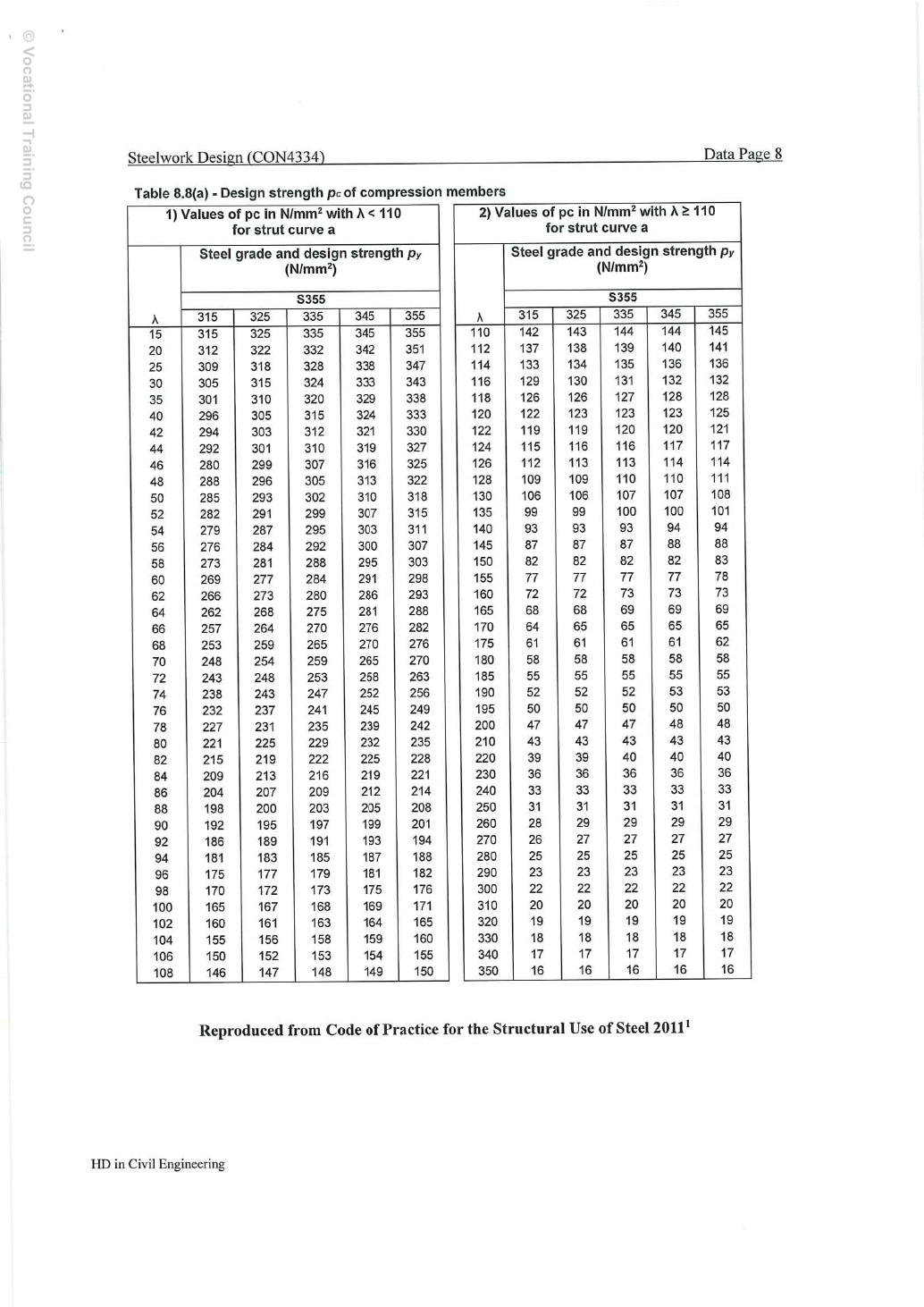
Table 8.8(a): design compressive strength for strut curve a. Both left and right halves use strength units ; the S355 columns are, in order, . The left half is labelled , with printed rows from to ; the right half is labelled , with printed rows from to . Row spacing changes: find the actual two rows bracketing the required value instead of assuming a fixed interval. Interpolate only within one curve and design-strength column. The page credits the Hong Kong 2011 steel code; its footer identifies HD in Civil Engineering.
Animation labEffective length and buckling axes
Supplement to the original lesson. Enable JavaScript to play, step through calculations and rotate 3D models. The following explanation remains readable offline.
- A column can bow sideways before its section reaches the crushing resistance.
- Each axis has its own radius of gyration and restraint spacing.
- , with compatible length units. A tie affects only the directions it actually restrains.
- Select each buckling curve and compressive strength before forming Pc. The governing axis is determined by resistance, not slenderness alone.
2023 attachment 9: Compression curve b
This is printed Data page 9, physical PDF page 15, in Pastpaper/22ENGTY033.pdf. Use three keys: curve, material design strength and . If curve c, and , rows / give /; . With , . Repeat for the other axis and retain the governing resistance. Data File curve b, py 355, λ90 prints “”; the full lecture Ch 4 p 8 clearly gives , which this site uses. Unlike the compact standalone sheet, this page also supplies the high-slenderness half (). Select the correct half before bracketing; the last low-range row is not a licence to extrapolate.
Detailed lookup rules and units.
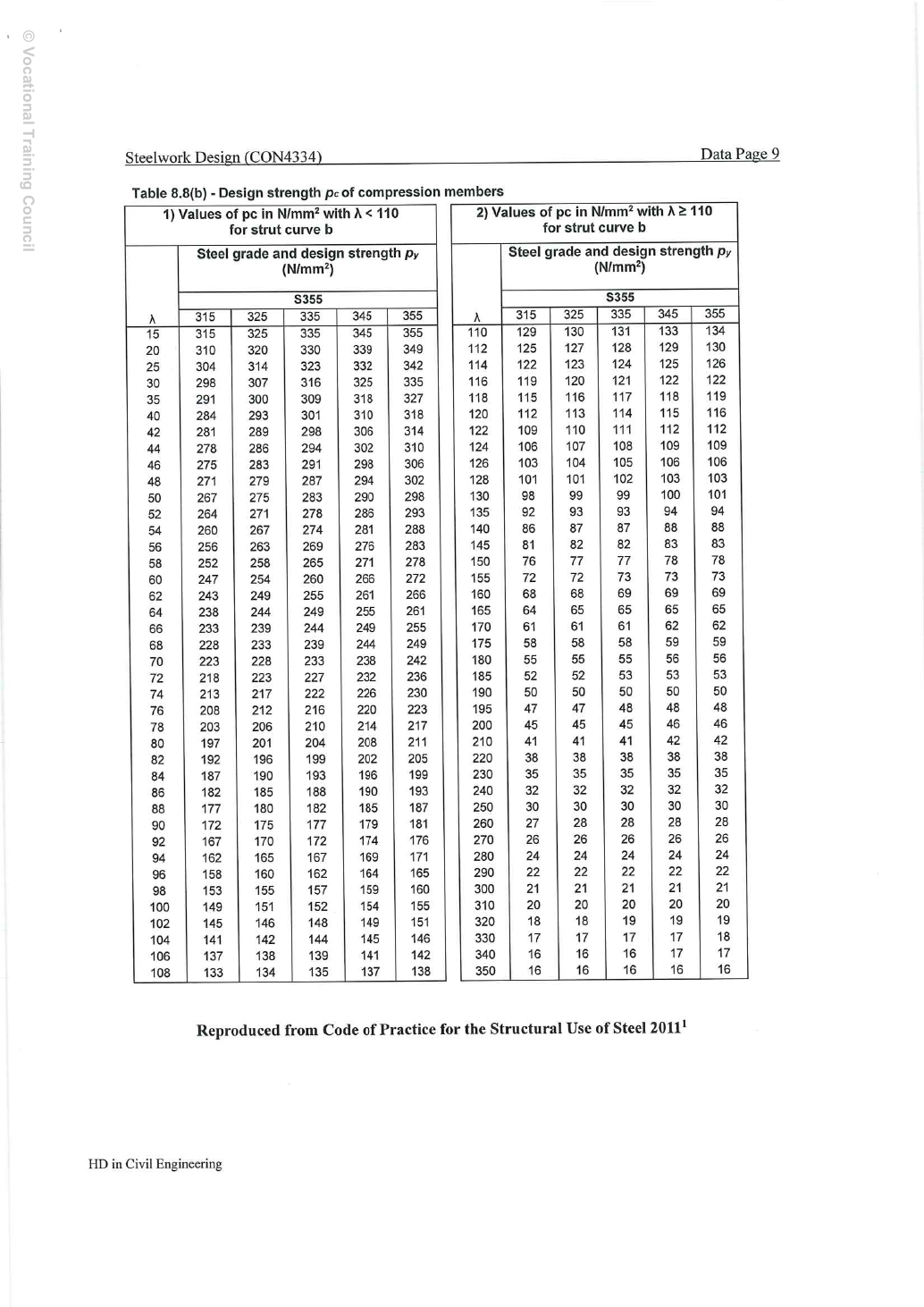
Table 8.8(b): design compressive strength for strut curve b. Both left and right halves use strength units ; the S355 columns are, in order, . The left half is labelled , with printed rows from to ; the right half is labelled , with printed rows from to . Row spacing changes: find the actual bracketing rows instead of assuming a fixed interval. Interpolate only within one curve and design-strength column. This exam gives , of , distinct from the separate Data File's misprinted . The page credits the Hong Kong 2011 steel code; its footer identifies HD in Civil Engineering.
Animation labEffective length and buckling axes
Supplement to the original lesson. Enable JavaScript to play, step through calculations and rotate 3D models. The following explanation remains readable offline.
- A column can bow sideways before its section reaches the crushing resistance.
- Each axis has its own radius of gyration and restraint spacing.
- , with compatible length units. A tie affects only the directions it actually restrains.
- Select each buckling curve and compressive strength before forming Pc. The governing axis is determined by resistance, not slenderness alone.
2023 attachment 10: Compression curve c
This is printed Data page 10, physical PDF page 16, in Pastpaper/22ENGTY033.pdf. Use three keys: curve, material design strength and . If curve c, and , rows / give /; . With , . Repeat for the other axis and retain the governing resistance. Data File curve b, py 355, λ90 prints “”; the full lecture Ch 4 p 8 clearly gives , which this site uses. Unlike the compact standalone sheet, this page also supplies the high-slenderness half (). Select the correct half before bracketing; the last low-range row is not a licence to extrapolate.
Detailed lookup rules and units.
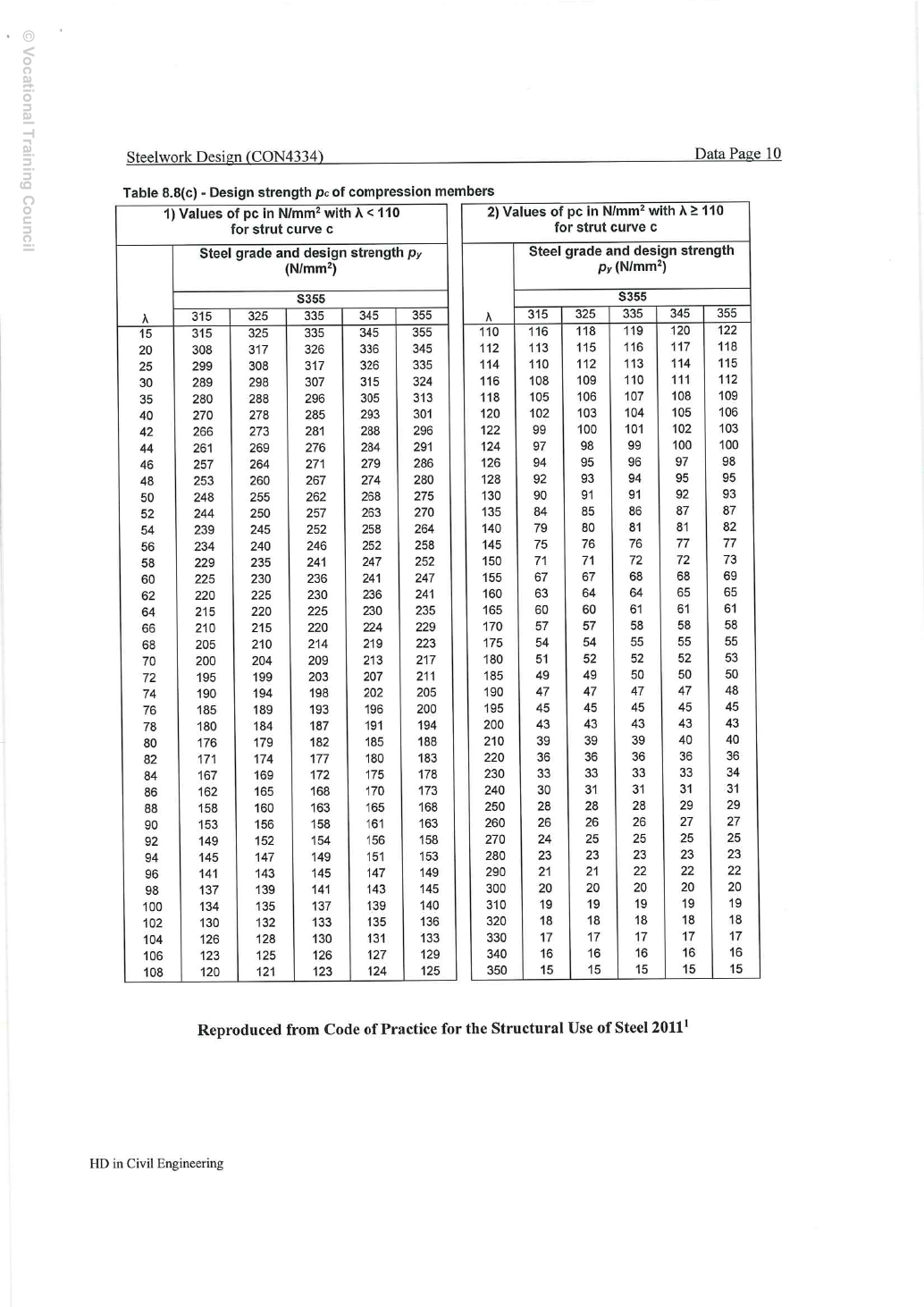
Table 8.8(c): design compressive strength for strut curve c. Both left and right halves use strength units ; the S355 columns are, in order, . The left half is labelled , with printed rows from to ; the right half is labelled , with printed rows from to . Row spacing changes: find the actual two rows bracketing the required value instead of assuming a fixed interval. Interpolate only within one curve and design-strength column. The page credits the Hong Kong 2011 steel code; its footer identifies HD in Civil Engineering.
Animation labEffective length and buckling axes
Supplement to the original lesson. Enable JavaScript to play, step through calculations and rotate 3D models. The following explanation remains readable offline.
- A column can bow sideways before its section reaches the crushing resistance.
- Each axis has its own radius of gyration and restraint spacing.
- , with compatible length units. A tie affects only the directions it actually restrains.
- Select each buckling curve and compressive strength before forming Pc. The governing axis is determined by resistance, not slenderness alone.
2023 attachment 11: Compression curve d
This is printed Data page 11, physical PDF page 17, in Pastpaper/22ENGTY033.pdf. Use three keys: curve, material design strength and . If curve c, and , rows / give /; . With , . Repeat for the other axis and retain the governing resistance. Data File curve b, py 355, λ90 prints “”; the full lecture Ch 4 p 8 clearly gives , which this site uses. Unlike the compact standalone sheet, this page also supplies the high-slenderness half (). Select the correct half before bracketing; the last low-range row is not a licence to extrapolate.
Detailed lookup rules and units.
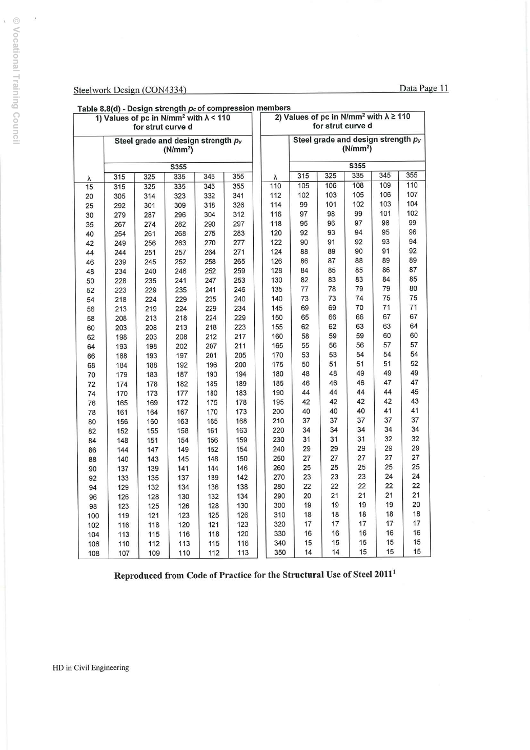
Table 8.8(d): design compressive strength for strut curve d. Both left and right halves use strength units ; the S355 columns are, in order, . The left half is labelled , with printed rows from to ; the right half is labelled , with printed rows from to . Row spacing changes: find the actual two rows bracketing the required value instead of assuming a fixed interval. Interpolate only within one curve and design-strength column. The page credits the Hong Kong 2011 steel code; its footer identifies HD in Civil Engineering.
Animation labEffective length and buckling axes
Supplement to the original lesson. Enable JavaScript to play, step through calculations and rotate 3D models. The following explanation remains readable offline.
- A column can bow sideways before its section reaches the crushing resistance.
- Each axis has its own radius of gyration and restraint spacing.
- , with compatible length units. A tie affects only the directions it actually restrains.
- Select each buckling curve and compressive strength before forming Pc. The governing axis is determined by resistance, not slenderness alone.
2023 attachment 12: Larger UB dimensions
This is printed Data page 12, physical PDF page 18, in Pastpaper/22ENGTY033.pdf. Match all three designation numbers, including mass. Read actual depth , width , web , flange , root radius , clear web depth and tabulated ,. The nominal name does not mean its exact depth is or its web is thick. Dimension-table is not bolt diameter; its meaning changes with context. A larger flange thickness can lower and must be checked after selection. Dimensions and properties are on paired pages: 12 with 13, and 14 with 15. Match the complete designation again after turning the page.
Detailed lookup rules and units.
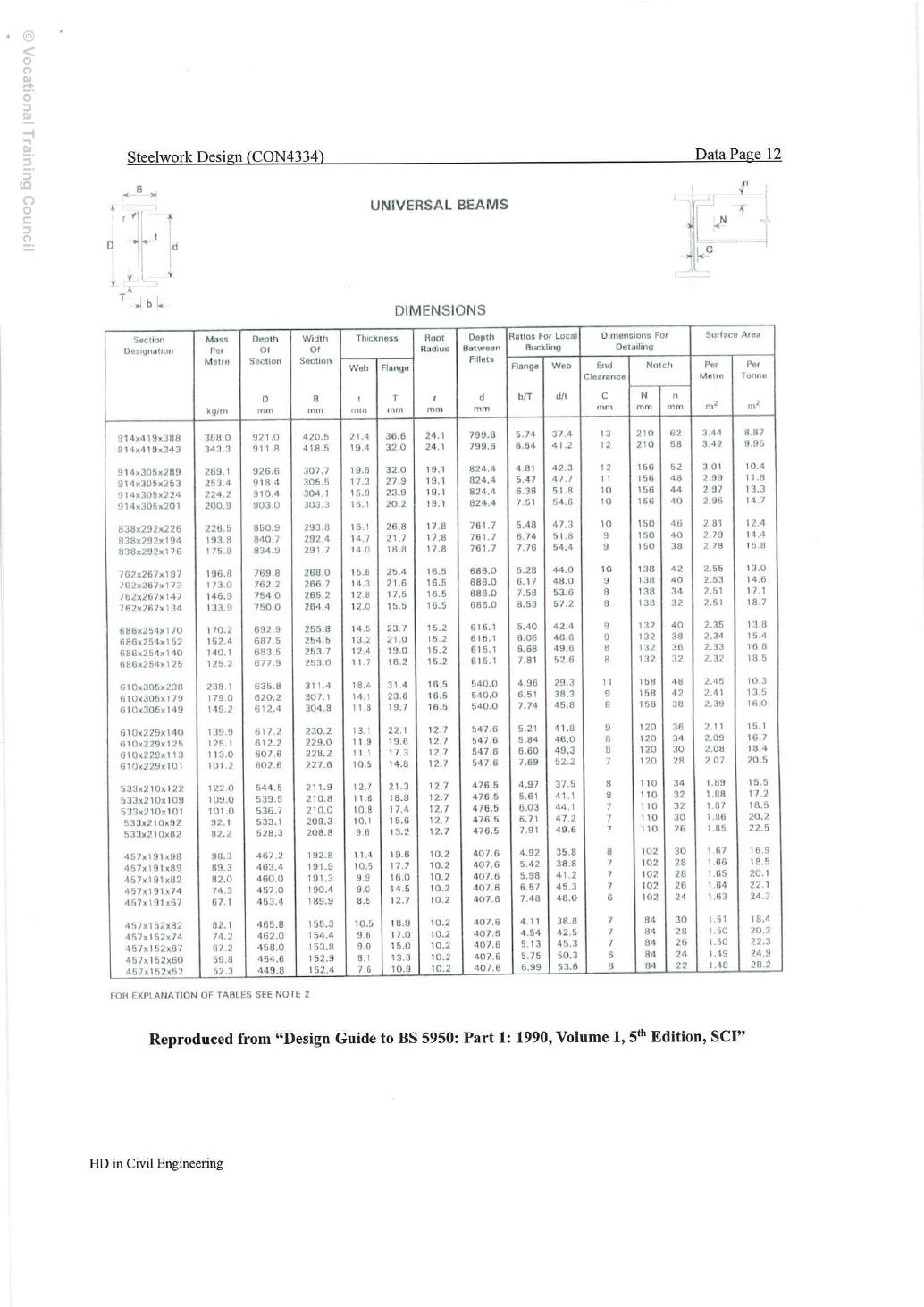
UNIVERSAL BEAMS / DIMENSIONS. In the upper-left section sketch, spans overall section depth; spans full flange width; crosses web thickness; crosses flange thickness; points to the root fillet; spans clear web depth between root fillets; is the flange outstand width shown. Classification still uses the tabulated ratios. In the upper-right notch sketch, is end clearance; is horizontal notch dimension; is vertical notch dimension. This is not the question's load diagram and specifies no actual beam length.
Column headings: Section Designation; Mass Per Metre, ; Depth / Width / Web / Flange / Root Radius / Depth Between Fillets correspond respectively to , , , , , , all in ; Ratios for Local Buckling give flange and web , both dimensionless; Dimensions for Detailing, , , uses . Finally, the two Surface Area columns are per metre and per tonne, in . The source page credits Design Guide to BS 5950: Part 1: 1990, Volume 1, 5th Edition, SCI as the publication source of the supplied section tables. The design method still follows the course Hong Kong code.
Source headings, dimension/axis sketches and units on this page have been matched individually. The table directs the reader to Note 2. Matching legends does not imply that every numerical cell is identical across different appendices. Cite the actual page and complete section row used in a calculation.
Animation labExplore section geometry and axes
Supplement to the original lesson. Enable JavaScript to play, step through calculations and rotate 3D models. The following explanation remains readable offline.
- The flanges are the wide plates; the web connects them. Rotate the I-section to see both.
- The same section has different stiffness and resistance about its two principal axes.
- I controls elastic curvature; is elastic section modulus. Plastic modulus S comes from plastic stress blocks.
- Nominal section labels are not every actual dimension. Keep the row, axis and units together.
2023 attachment 13: Larger UB properties
This is printed Data page 13, physical PDF page 19, in Pastpaper/22ENGTY033.pdf. Use the same complete section designation as the dimension table. Read , in (×→), , in (×→), , and , in (×→), area in (×→), plus dimensionless and torsional index . Use for major-axis vertical deflection, for LTB slenderness, for Class 1/2 bending and elastic for the specified column member equations. Never interpolate between different section sizes to create a fictional section. Dimensions and properties are on paired pages: 12 with 13, and 14 with 15. Match the complete designation again after turning the page.
Detailed lookup rules and units.
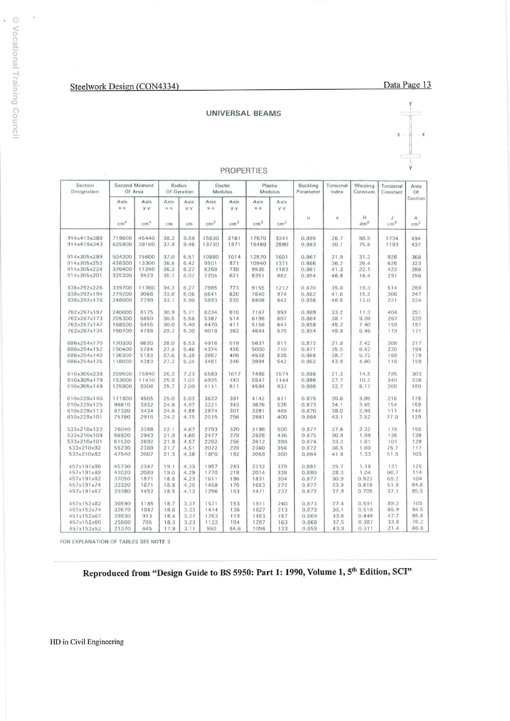
UNIVERSAL BEAMS / PROPERTIES. In the upper-right sketch, horizontal is the major axis and vertical is the minor axis, both through the centroid. No applied load is shown. Columns give Second Moment of Area, in order , (); Radius of Gyration, , (); Elastic Modulus, , (); Plastic Modulus, , (). Here Modulus means section modulus, not the material's Young's modulus.
Buckling Parameter ; Torsional Index , not the axis; Warping Constant (source table ); Torsional Constant (); Area of Section (). This is the section's torsional constant, not the line-weld group polar inertia . The source page is extracted from Design Guide to BS 5950: Part 1: 1990, Volume 1, 5th Edition, SCI; all selected properties must belong to the same section row.
Source headings, dimension/axis sketches and units on this page have been matched individually. The table directs the reader to Note 3. Matching legends does not imply that every numerical cell is identical across different appendices. Cite the actual page and complete section row used in a calculation.
Animation labExplore section geometry and axes
Supplement to the original lesson. Enable JavaScript to play, step through calculations and rotate 3D models. The following explanation remains readable offline.
- The flanges are the wide plates; the web connects them. Rotate the I-section to see both.
- The same section has different stiffness and resistance about its two principal axes.
- I controls elastic curvature; is elastic section modulus. Plastic modulus S comes from plastic stress blocks.
- Nominal section labels are not every actual dimension. Keep the row, axis and units together.
2023 attachment 14: Smaller UB dimensions
This is printed Data page 14, physical PDF page 20, in Pastpaper/22ENGTY033.pdf. Match all three designation numbers, including mass. Read actual depth , width , web , flange , root radius , clear web depth and tabulated ,. The nominal name does not mean its exact depth is or its web is thick. Dimension-table is not bolt diameter; its meaning changes with context. A larger flange thickness can lower and must be checked after selection. Dimensions and properties are on paired pages: 12 with 13, and 14 with 15. Match the complete designation again after turning the page.
Detailed lookup rules and units.
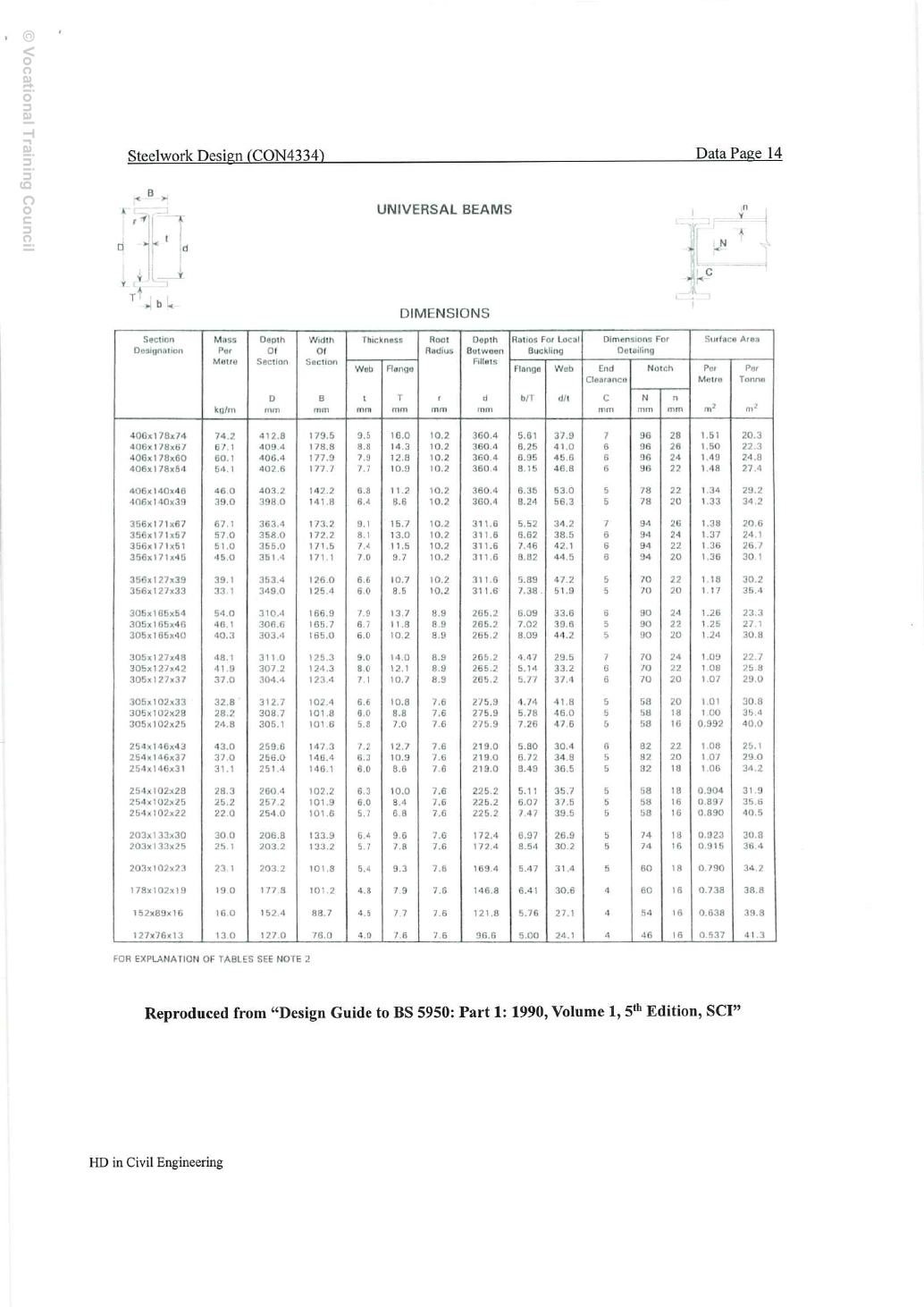
UNIVERSAL BEAMS / DIMENSIONS. In the upper-left section sketch, spans overall section depth; spans full flange width; crosses web thickness; crosses flange thickness; points to the root fillet; spans clear web depth between root fillets; is the flange outstand width shown. Classification still uses the tabulated ratios. In the upper-right notch sketch, is end clearance; is horizontal notch dimension; is vertical notch dimension. This is not the question's load diagram and specifies no actual beam length.
Column headings: Section Designation; Mass Per Metre, ; Depth / Width / Web / Flange / Root Radius / Depth Between Fillets correspond respectively to , , , , , , all in ; Ratios for Local Buckling give flange and web , both dimensionless; Dimensions for Detailing, , , uses . Finally, the two Surface Area columns are per metre and per tonne, in . The source page credits Design Guide to BS 5950: Part 1: 1990, Volume 1, 5th Edition, SCI as the publication source of the supplied section tables. The design method still follows the course Hong Kong code.
Source headings, dimension/axis sketches and units on this page have been matched individually. The table directs the reader to Note 2. Matching legends does not imply that every numerical cell is identical across different appendices. Cite the actual page and complete section row used in a calculation.
Animation labExplore section geometry and axes
Supplement to the original lesson. Enable JavaScript to play, step through calculations and rotate 3D models. The following explanation remains readable offline.
- The flanges are the wide plates; the web connects them. Rotate the I-section to see both.
- The same section has different stiffness and resistance about its two principal axes.
- I controls elastic curvature; is elastic section modulus. Plastic modulus S comes from plastic stress blocks.
- Nominal section labels are not every actual dimension. Keep the row, axis and units together.
2023 attachment 15: Smaller UB properties
This is printed Data page 15, physical PDF page 21, in Pastpaper/22ENGTY033.pdf. Use the same complete section designation as the dimension table. Read , in (×→), , in (×→), , and , in (×→), area in (×→), plus dimensionless and torsional index . Use for major-axis vertical deflection, for LTB slenderness, for Class 1/2 bending and elastic for the specified column member equations. Never interpolate between different section sizes to create a fictional section. Dimensions and properties are on paired pages: 12 with 13, and 14 with 15. Match the complete designation again after turning the page.
Detailed lookup rules and units.
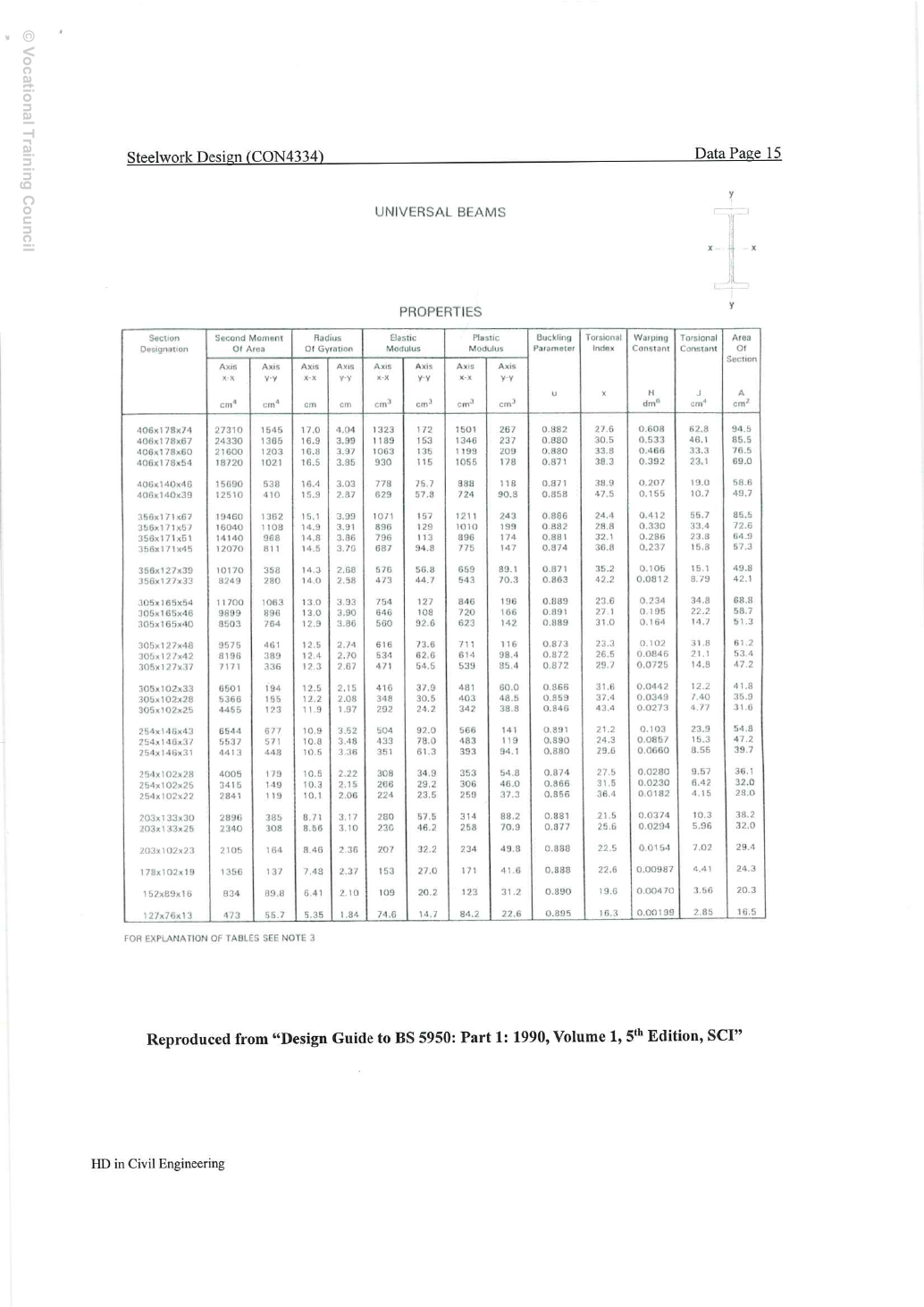
UNIVERSAL BEAMS / PROPERTIES. In the upper-right sketch, horizontal is the major axis and vertical is the minor axis, both through the centroid. No applied load is shown. Columns give Second Moment of Area, in order , (); Radius of Gyration, , (); Elastic Modulus, , (); Plastic Modulus, , (). Here Modulus means section modulus, not the material's Young's modulus.
Buckling Parameter ; Torsional Index , not the axis; Warping Constant (source table ); Torsional Constant (); Area of Section (). This is the section's torsional constant, not the line-weld group polar inertia . The source page is extracted from Design Guide to BS 5950: Part 1: 1990, Volume 1, 5th Edition, SCI; all selected properties must belong to the same section row.
Source headings, dimension/axis sketches and units on this page have been matched individually. The table directs the reader to Note 3. Matching legends does not imply that every numerical cell is identical across different appendices. Cite the actual page and complete section row used in a calculation.
Animation labExplore section geometry and axes
Supplement to the original lesson. Enable JavaScript to play, step through calculations and rotate 3D models. The following explanation remains readable offline.
- The flanges are the wide plates; the web connects them. Rotate the I-section to see both.
- The same section has different stiffness and resistance about its two principal axes.
- I controls elastic curvature; is elastic section modulus. Plastic modulus S comes from plastic stress blocks.
- Nominal section labels are not every actual dimension. Keep the row, axis and units together.
2023 attachment 16: UC dimensions
Source: Pastpaper/22ENGTY033.pdf, printed Data p.16 / physical PDF p.22. The comparison below contrasts this exam with the separate Data File. “Not on this page” refers to the separate data page; exam Data pp.16–17 are the source of the larger UC. The separate data page combines UC dimensions and properties. Read one exactly matching section row, then roughly check whether is consistent with mass per metre. This only screens for transcription mistakes and does not replace tabulated values. The larger UC needed for Assignment 2 is absent from this page but is supplied in 2023 Data pp.16–17. That solution explicitly cites its lookup source.
Detailed lookup rules and units.
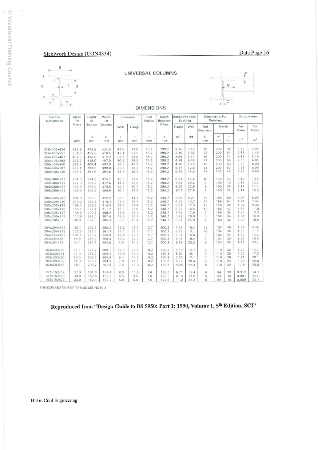
UNIVERSAL COLUMNS / DIMENSIONS. Upper-left section sketch: spans overall section depth; spans full flange width; crosses web thickness; crosses flange thickness; points to the root fillet; spans clear web depth between root fillets; is the flange outstand width shown. Classification still uses the tabulated ratios. In the upper-right notch sketch, is end clearance; is horizontal notch dimension; is vertical notch dimension. This is not the question's load diagram and specifies no actual beam length.
Column headings: Section Designation; Mass Per Metre, ; Depth / Width / Web / Flange / Root Radius / Depth Between Fillets correspond respectively to , , , , , , all in ; Ratios for Local Buckling give flange and web , both dimensionless; Dimensions for Detailing, , , uses . Finally, the two Surface Area columns are per metre and per tonne, in . The source page credits Design Guide to BS 5950: Part 1: 1990, Volume 1, 5th Edition, SCI as the publication source of the supplied section tables. The design method still follows the course Hong Kong code.
Source headings, dimension/axis sketches and units on this page have been matched individually. The table directs the reader to Note 2. Matching legends does not imply that every numerical cell is identical across different appendices. Cite the actual page and complete section row used in a calculation.
Animation labExplore section geometry and axes
Supplement to the original lesson. Enable JavaScript to play, step through calculations and rotate 3D models. The following explanation remains readable offline.
- The flanges are the wide plates; the web connects them. Rotate the I-section to see both.
- The same section has different stiffness and resistance about its two principal axes.
- I controls elastic curvature; is elastic section modulus. Plastic modulus S comes from plastic stress blocks.
- Nominal section labels are not every actual dimension. Keep the row, axis and units together.
2023 attachment 17: UC properties
Source: Pastpaper/22ENGTY033.pdf, printed Data p.17 / physical PDF p.23. The comparison below contrasts this exam with the separate Data File. “Not on this page” refers to the separate data page; exam Data pp.16–17 are the source of the larger UC. The separate data page combines UC dimensions and properties. Read one exactly matching section row, then roughly check whether is consistent with mass per metre. This only screens for transcription mistakes and does not replace tabulated values. The larger UC needed for Assignment 2 is absent from this page but is supplied in 2023 Data pp.16–17. That solution explicitly cites its lookup source.
Detailed lookup rules and units.
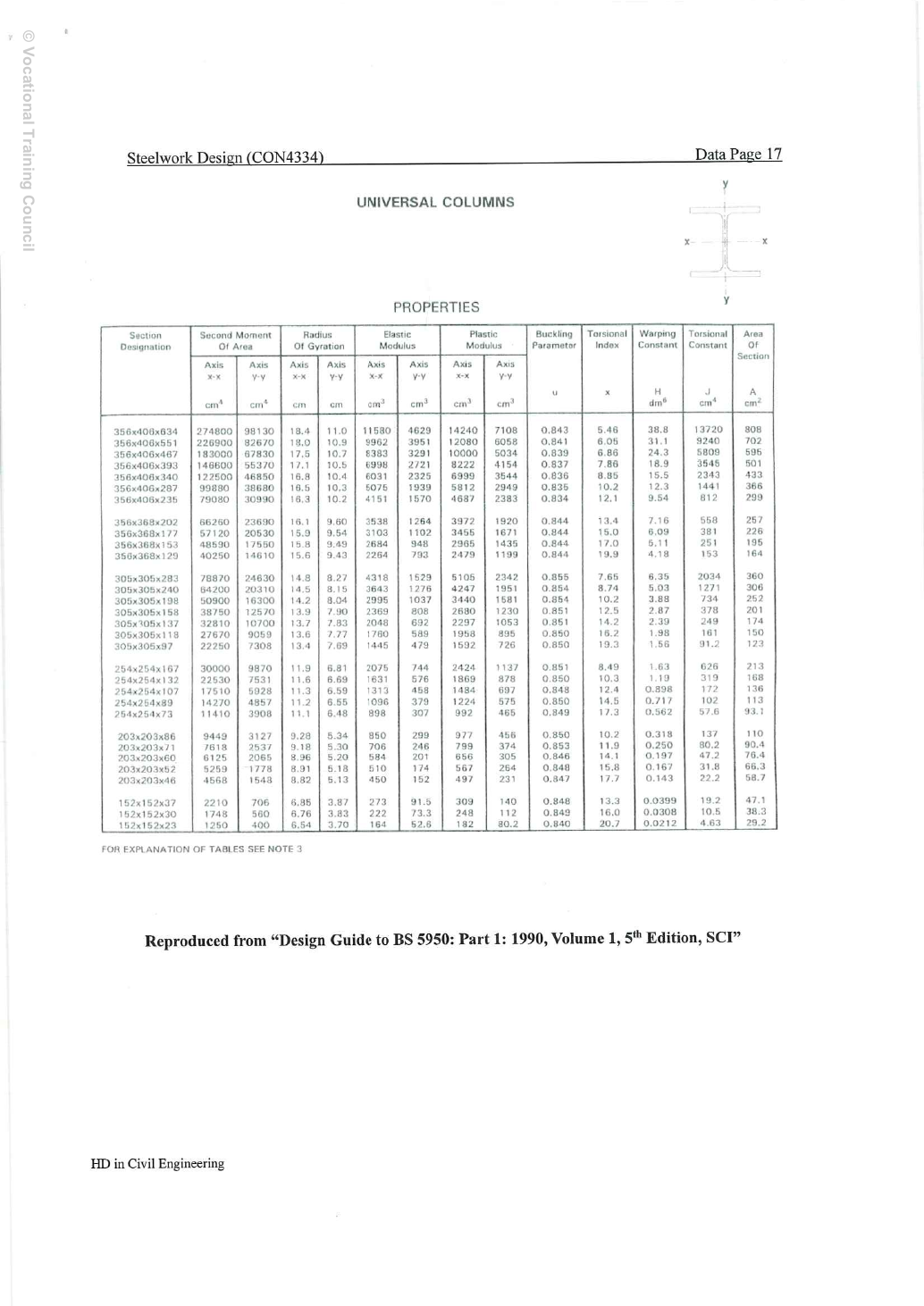
UNIVERSAL COLUMNS / PROPERTIES. In the upper-right sketch, horizontal is the major axis and vertical is the minor axis, both through the centroid. No applied load is shown. Columns give Second Moment of Area, in order , (); Radius of Gyration, , (); Elastic Modulus, , (); Plastic Modulus, , (). Here Modulus means section modulus, not the material's Young's modulus.
Buckling Parameter ; Torsional Index , not the axis; Warping Constant (source table ); Torsional Constant (); Area of Section (). This is the section's torsional constant, not the line-weld group polar inertia . The source page is extracted from Design Guide to BS 5950: Part 1: 1990, Volume 1, 5th Edition, SCI; all selected properties must belong to the same section row.
Source headings, dimension/axis sketches and units on this page have been matched individually. The table directs the reader to Note 3. Matching legends does not imply that every numerical cell is identical across different appendices. Cite the actual page and complete section row used in a calculation.
Animation labExplore section geometry and axes
Supplement to the original lesson. Enable JavaScript to play, step through calculations and rotate 3D models. The following explanation remains readable offline.
- The flanges are the wide plates; the web connects them. Rotate the I-section to see both.
- The same section has different stiffness and resistance about its two principal axes.
- I controls elastic curvature; is elastic section modulus. Plastic modulus S comes from plastic stress blocks.
- Nominal section labels are not every actual dimension. Keep the row, axis and units together.
2023 attachment 18: Unequal angles
This is printed Data page 18, physical PDF page 24, in Pastpaper/22ENGTY033.pdf. Match long leg, short leg and thickness; read the small axis sketch before selecting or . For an angle whose long leg is connected, the distance from heel to centroid along that leg determines balanced longitudinal weld forces. This is not generally half the leg length. The table includes rolled root effects; simple rectangular angle areas in worked questions are identified as that course approximation. The standalone block contains inconsistent thickness labels; do not borrow an uncertain area for the question.
Detailed lookup rules and units.
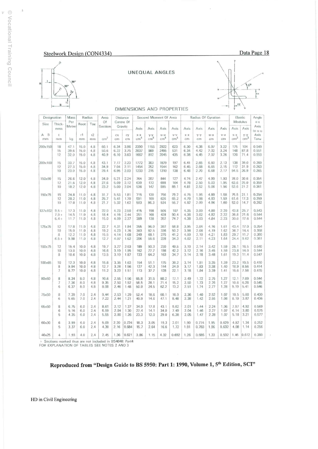
UNEQUAL ANGLES / DIMENSIONS AND PROPERTIES. Upper-left sketch: is the full vertical long-leg length; the full horizontal short-leg length; leg thickness; included angle , is the internal root radius; is the toe radius. Upper-right sketch: is horizontal; is vertical; they intersect at the centroid. is the vertical distance from the short leg's outer back to the horizontal centroidal axis; is the horizontal distance from the long leg's outer back to the vertical centroidal axis. Inclined axes , are the principal axes; is their shown rotation. A subscript does not make a horizontally measured distance.
This table includes principal-axis properties absent from the separate Data File angle table. Headings in order: dimensions , and thickness (); mass per metre (the source heading prints ; the per-metre meaning comes from Mass Per Metre); root and toe radii (); section area (); centroid distances , (). Second moments are listed about , , , (); radii of gyration follow the same order (); elastic section moduli are given only for , (). The final column Tan α means , the dimensionless tangent of the shown principal-axis rotation, not the angle itself.
The + after thickness is a source note identifying a section not included in BS4848: Part 4, not addition of dimensions. In this block, the thicknesses are, in order, , with a + on the final row. Do not conflate these with the inconsistent labels in the separate Data File. The table directs the reader to Notes 2 and 3. Source publication: Design Guide to BS 5950: Part 1: 1990, Volume 1, 5th Edition, SCI; the course's supplied sources and code method are retained.
Animation labWhy a connected angle leg matters
Supplement to the original lesson. Enable JavaScript to play, step through calculations and rotate 3D models. The following explanation remains readable offline.
- Locate the connected leg, outstanding leg and centroid before using the table.
- Only the connected leg directly receives the fastener force.
- The outstanding area may not become equally effective at the same section; this motivates the effective-area rule.
- Bolted, welded, single-angle and double-angle details can have different rules. Preserve the formula attached to the original case.
Rebuild every cell of the lecture bolt-capacity tables
Source: Ch 2 p 5, Tables 4 and 5. Each cell is stress×area÷. Tension always uses tensile stress area . Shank shear uses the tabulated rounded shank area ; thread shear uses . These are single-plane shear capacities and individual tension capacities. The examples below calculate from the printed input areas; the original tables sometimes round down rather than to nearest. Use unrounded arithmetic for subsequent comparisons.
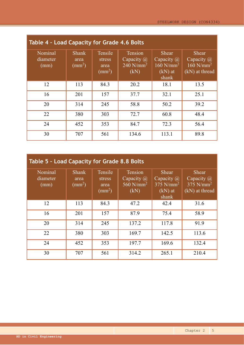
Table 4 is Grade 4.6; Table 5 is Grade 8.8. Nominal diameter (); Shank area and Tensile stress area (both in ). Tension Capacity and Shear Capacity at shank / at thread are all in . Grade 4.6 headings specify tensile stress and shear stress ; the Grade 8.8 values are respectively , . Each cell below retains both the original table value and the value calculated from its printed area. For example, the Grade 8.8 M24 shank-shear entry prints , whereas using the tabulated gives . Do not describe the two as equal.
Animation labCount the bolt shear planes
Supplement to the original lesson. Enable JavaScript to play, step through calculations and rotate 3D models. The following explanation remains readable offline.
- Load must cross an interface between the connected plates.
- A lap joint gives one shear plane through a bolt.
- A symmetric double-cover joint may provide two shear planes. Count load-transfer interfaces, not just visible plates.
- Use the source’s area and shear strength. Then check bearing, plate resistance and detailing separately.
Grade 4.6, M12: all three cells
Given row M12: and . Lookup grade 4.6: and . Required: individual tensile resistance and the two possible single-plane shear resistances.
Tension. Multiply applicable area by design stress to obtain , then divide by for .
Original printed cell: .
Unthreaded shank shear. Multiply applicable area by design stress to obtain , then divide by for .
Original printed cell: .
Thread shear. Multiply applicable area by design stress to obtain , then divide by for .
Original printed cell: .
Try it yourself. For two threaded shear planes through this M12 bolt, what is total shear resistance?
Reveal answer and reasoning
. This doubles shear planes, not tensile resistance or every bearing limit.
Animation labCount the bolt shear planes
Supplement to the original lesson. Enable JavaScript to play, step through calculations and rotate 3D models. The following explanation remains readable offline.
- Load must cross an interface between the connected plates.
- A lap joint gives one shear plane through a bolt.
- A symmetric double-cover joint may provide two shear planes. Count load-transfer interfaces, not just visible plates.
- Use the source’s area and shear strength. Then check bearing, plate resistance and detailing separately.
Animation labCount the bolt shear planes
Supplement to the original lesson. Enable JavaScript to play, step through calculations and rotate 3D models. The following explanation remains readable offline.
- Load must cross an interface between the connected plates.
- A lap joint gives one shear plane through a bolt.
- A symmetric double-cover joint may provide two shear planes. Count load-transfer interfaces, not just visible plates.
- Use the source’s area and shear strength. Then check bearing, plate resistance and detailing separately.
Grade 4.6, M16: all three cells
Given row M16: and . Lookup grade 4.6: and . Required: individual tensile resistance and the two possible single-plane shear resistances.
Tension. Multiply applicable area by design stress to obtain , then divide by for .
Original printed cell: .
Unthreaded shank shear. Multiply applicable area by design stress to obtain , then divide by for .
Original printed cell: .
Thread shear. Multiply applicable area by design stress to obtain , then divide by for .
Original printed cell: .
Try it yourself. For two threaded shear planes through this M16 bolt, what is total shear resistance?
Reveal answer and reasoning
. This doubles shear planes, not tensile resistance or every bearing limit.
Animation labCount the bolt shear planes
Supplement to the original lesson. Enable JavaScript to play, step through calculations and rotate 3D models. The following explanation remains readable offline.
- Load must cross an interface between the connected plates.
- A lap joint gives one shear plane through a bolt.
- A symmetric double-cover joint may provide two shear planes. Count load-transfer interfaces, not just visible plates.
- Use the source’s area and shear strength. Then check bearing, plate resistance and detailing separately.
Animation labCount the bolt shear planes
Supplement to the original lesson. Enable JavaScript to play, step through calculations and rotate 3D models. The following explanation remains readable offline.
- Load must cross an interface between the connected plates.
- A lap joint gives one shear plane through a bolt.
- A symmetric double-cover joint may provide two shear planes. Count load-transfer interfaces, not just visible plates.
- Use the source’s area and shear strength. Then check bearing, plate resistance and detailing separately.
Grade 4.6, M20: all three cells
Given row M20: and . Lookup grade 4.6: and . Required: individual tensile resistance and the two possible single-plane shear resistances.
Tension. Multiply applicable area by design stress to obtain , then divide by for .
Original printed cell: .
Unthreaded shank shear. Multiply applicable area by design stress to obtain , then divide by for .
Original printed cell: .
Thread shear. Multiply applicable area by design stress to obtain , then divide by for .
Original printed cell: .
Try it yourself. For two threaded shear planes through this M20 bolt, what is total shear resistance?
Reveal answer and reasoning
. This doubles shear planes, not tensile resistance or every bearing limit.
Animation labCount the bolt shear planes
Supplement to the original lesson. Enable JavaScript to play, step through calculations and rotate 3D models. The following explanation remains readable offline.
- Load must cross an interface between the connected plates.
- A lap joint gives one shear plane through a bolt.
- A symmetric double-cover joint may provide two shear planes. Count load-transfer interfaces, not just visible plates.
- Use the source’s area and shear strength. Then check bearing, plate resistance and detailing separately.
Animation labCount the bolt shear planes
Supplement to the original lesson. Enable JavaScript to play, step through calculations and rotate 3D models. The following explanation remains readable offline.
- Load must cross an interface between the connected plates.
- A lap joint gives one shear plane through a bolt.
- A symmetric double-cover joint may provide two shear planes. Count load-transfer interfaces, not just visible plates.
- Use the source’s area and shear strength. Then check bearing, plate resistance and detailing separately.
Grade 4.6, M22: all three cells
Given row M22: and . Lookup grade 4.6: and . Required: individual tensile resistance and the two possible single-plane shear resistances.
Tension. Multiply applicable area by design stress to obtain , then divide by for .
Original printed cell: .
Unthreaded shank shear. Multiply applicable area by design stress to obtain , then divide by for .
Original printed cell: .
Thread shear. Multiply applicable area by design stress to obtain , then divide by for .
Original printed cell: .
Try it yourself. For two threaded shear planes through this M22 bolt, what is total shear resistance?
Reveal answer and reasoning
. This doubles shear planes, not tensile resistance or every bearing limit.
Animation labCount the bolt shear planes
Supplement to the original lesson. Enable JavaScript to play, step through calculations and rotate 3D models. The following explanation remains readable offline.
- Load must cross an interface between the connected plates.
- A lap joint gives one shear plane through a bolt.
- A symmetric double-cover joint may provide two shear planes. Count load-transfer interfaces, not just visible plates.
- Use the source’s area and shear strength. Then check bearing, plate resistance and detailing separately.
Animation labCount the bolt shear planes
Supplement to the original lesson. Enable JavaScript to play, step through calculations and rotate 3D models. The following explanation remains readable offline.
- Load must cross an interface between the connected plates.
- A lap joint gives one shear plane through a bolt.
- A symmetric double-cover joint may provide two shear planes. Count load-transfer interfaces, not just visible plates.
- Use the source’s area and shear strength. Then check bearing, plate resistance and detailing separately.
Grade 4.6, M24: all three cells
Given row M24: and . Lookup grade 4.6: and . Required: individual tensile resistance and the two possible single-plane shear resistances.
Tension. Multiply applicable area by design stress to obtain , then divide by for .
Original printed cell: .
Unthreaded shank shear. Multiply applicable area by design stress to obtain , then divide by for .
Original printed cell: .
Thread shear. Multiply applicable area by design stress to obtain , then divide by for .
Original printed cell: .
Try it yourself. For two threaded shear planes through this M24 bolt, what is total shear resistance?
Reveal answer and reasoning
. This doubles shear planes, not tensile resistance or every bearing limit.
Animation labCount the bolt shear planes
Supplement to the original lesson. Enable JavaScript to play, step through calculations and rotate 3D models. The following explanation remains readable offline.
- Load must cross an interface between the connected plates.
- A lap joint gives one shear plane through a bolt.
- A symmetric double-cover joint may provide two shear planes. Count load-transfer interfaces, not just visible plates.
- Use the source’s area and shear strength. Then check bearing, plate resistance and detailing separately.
Animation labCount the bolt shear planes
Supplement to the original lesson. Enable JavaScript to play, step through calculations and rotate 3D models. The following explanation remains readable offline.
- Load must cross an interface between the connected plates.
- A lap joint gives one shear plane through a bolt.
- A symmetric double-cover joint may provide two shear planes. Count load-transfer interfaces, not just visible plates.
- Use the source’s area and shear strength. Then check bearing, plate resistance and detailing separately.
Grade 4.6, M30: all three cells
Given row M30: and . Lookup grade 4.6: and . Required: individual tensile resistance and the two possible single-plane shear resistances.
Tension. Multiply applicable area by design stress to obtain , then divide by for .
Original printed cell: .
Unthreaded shank shear. Multiply applicable area by design stress to obtain , then divide by for .
Original printed cell: .
Thread shear. Multiply applicable area by design stress to obtain , then divide by for .
Original printed cell: .
Try it yourself. For two threaded shear planes through this M30 bolt, what is total shear resistance?
Reveal answer and reasoning
. This doubles shear planes, not tensile resistance or every bearing limit.
Animation labCount the bolt shear planes
Supplement to the original lesson. Enable JavaScript to play, step through calculations and rotate 3D models. The following explanation remains readable offline.
- Load must cross an interface between the connected plates.
- A lap joint gives one shear plane through a bolt.
- A symmetric double-cover joint may provide two shear planes. Count load-transfer interfaces, not just visible plates.
- Use the source’s area and shear strength. Then check bearing, plate resistance and detailing separately.
Animation labCount the bolt shear planes
Supplement to the original lesson. Enable JavaScript to play, step through calculations and rotate 3D models. The following explanation remains readable offline.
- Load must cross an interface between the connected plates.
- A lap joint gives one shear plane through a bolt.
- A symmetric double-cover joint may provide two shear planes. Count load-transfer interfaces, not just visible plates.
- Use the source’s area and shear strength. Then check bearing, plate resistance and detailing separately.
Grade 8.8, M12: all three cells
Given row M12: and . Lookup grade 8.8: and . Required: individual tensile resistance and the two possible single-plane shear resistances.
Tension. Multiply applicable area by design stress to obtain , then divide by for .
Original printed cell: .
Unthreaded shank shear. Multiply applicable area by design stress to obtain , then divide by for .
Original printed cell: .
Thread shear. Multiply applicable area by design stress to obtain , then divide by for .
Original printed cell: .
Try it yourself. For two threaded shear planes through this M12 bolt, what is total shear resistance?
Reveal answer and reasoning
. This doubles shear planes, not tensile resistance or every bearing limit.
Animation labCount the bolt shear planes
Supplement to the original lesson. Enable JavaScript to play, step through calculations and rotate 3D models. The following explanation remains readable offline.
- Load must cross an interface between the connected plates.
- A lap joint gives one shear plane through a bolt.
- A symmetric double-cover joint may provide two shear planes. Count load-transfer interfaces, not just visible plates.
- Use the source’s area and shear strength. Then check bearing, plate resistance and detailing separately.
Animation labCount the bolt shear planes
Supplement to the original lesson. Enable JavaScript to play, step through calculations and rotate 3D models. The following explanation remains readable offline.
- Load must cross an interface between the connected plates.
- A lap joint gives one shear plane through a bolt.
- A symmetric double-cover joint may provide two shear planes. Count load-transfer interfaces, not just visible plates.
- Use the source’s area and shear strength. Then check bearing, plate resistance and detailing separately.
Grade 8.8, M16: all three cells
Given row M16: and . Lookup grade 8.8: and . Required: individual tensile resistance and the two possible single-plane shear resistances.
Tension. Multiply applicable area by design stress to obtain , then divide by for .
Original printed cell: .
Unthreaded shank shear. Multiply applicable area by design stress to obtain , then divide by for .
Original printed cell: .
Thread shear. Multiply applicable area by design stress to obtain , then divide by for .
Original printed cell: .
Try it yourself. For two threaded shear planes through this M16 bolt, what is total shear resistance?
Reveal answer and reasoning
. This doubles shear planes, not tensile resistance or every bearing limit.
Animation labCount the bolt shear planes
Supplement to the original lesson. Enable JavaScript to play, step through calculations and rotate 3D models. The following explanation remains readable offline.
- Load must cross an interface between the connected plates.
- A lap joint gives one shear plane through a bolt.
- A symmetric double-cover joint may provide two shear planes. Count load-transfer interfaces, not just visible plates.
- Use the source’s area and shear strength. Then check bearing, plate resistance and detailing separately.
Animation labCount the bolt shear planes
Supplement to the original lesson. Enable JavaScript to play, step through calculations and rotate 3D models. The following explanation remains readable offline.
- Load must cross an interface between the connected plates.
- A lap joint gives one shear plane through a bolt.
- A symmetric double-cover joint may provide two shear planes. Count load-transfer interfaces, not just visible plates.
- Use the source’s area and shear strength. Then check bearing, plate resistance and detailing separately.
Grade 8.8, M20: all three cells
Given row M20: and . Lookup grade 8.8: and . Required: individual tensile resistance and the two possible single-plane shear resistances.
Tension. Multiply applicable area by design stress to obtain , then divide by for .
Original printed cell: .
Unthreaded shank shear. Multiply applicable area by design stress to obtain , then divide by for .
Original printed cell: .
Thread shear. Multiply applicable area by design stress to obtain , then divide by for .
Original printed cell: .
Try it yourself. For two threaded shear planes through this M20 bolt, what is total shear resistance?
Reveal answer and reasoning
. This doubles shear planes, not tensile resistance or every bearing limit.
Animation labCount the bolt shear planes
Supplement to the original lesson. Enable JavaScript to play, step through calculations and rotate 3D models. The following explanation remains readable offline.
- Load must cross an interface between the connected plates.
- A lap joint gives one shear plane through a bolt.
- A symmetric double-cover joint may provide two shear planes. Count load-transfer interfaces, not just visible plates.
- Use the source’s area and shear strength. Then check bearing, plate resistance and detailing separately.
Animation labCount the bolt shear planes
Supplement to the original lesson. Enable JavaScript to play, step through calculations and rotate 3D models. The following explanation remains readable offline.
- Load must cross an interface between the connected plates.
- A lap joint gives one shear plane through a bolt.
- A symmetric double-cover joint may provide two shear planes. Count load-transfer interfaces, not just visible plates.
- Use the source’s area and shear strength. Then check bearing, plate resistance and detailing separately.
Grade 8.8, M22: all three cells
Given row M22: and . Lookup grade 8.8: and . Required: individual tensile resistance and the two possible single-plane shear resistances.
Tension. Multiply applicable area by design stress to obtain , then divide by for .
Original printed cell: .
Unthreaded shank shear. Multiply applicable area by design stress to obtain , then divide by for .
Original printed cell: .
Thread shear. Multiply applicable area by design stress to obtain , then divide by for .
Original printed cell: .
Try it yourself. For two threaded shear planes through this M22 bolt, what is total shear resistance?
Reveal answer and reasoning
. This doubles shear planes, not tensile resistance or every bearing limit.
Animation labCount the bolt shear planes
Supplement to the original lesson. Enable JavaScript to play, step through calculations and rotate 3D models. The following explanation remains readable offline.
- Load must cross an interface between the connected plates.
- A lap joint gives one shear plane through a bolt.
- A symmetric double-cover joint may provide two shear planes. Count load-transfer interfaces, not just visible plates.
- Use the source’s area and shear strength. Then check bearing, plate resistance and detailing separately.
Animation labCount the bolt shear planes
Supplement to the original lesson. Enable JavaScript to play, step through calculations and rotate 3D models. The following explanation remains readable offline.
- Load must cross an interface between the connected plates.
- A lap joint gives one shear plane through a bolt.
- A symmetric double-cover joint may provide two shear planes. Count load-transfer interfaces, not just visible plates.
- Use the source’s area and shear strength. Then check bearing, plate resistance and detailing separately.
Grade 8.8, M24: all three cells
Given row M24: and . Lookup grade 8.8: and . Required: individual tensile resistance and the two possible single-plane shear resistances.
Tension. Multiply applicable area by design stress to obtain , then divide by for .
Original printed cell: .
Unthreaded shank shear. Multiply applicable area by design stress to obtain , then divide by for .
Original printed cell: .
Thread shear. Multiply applicable area by design stress to obtain , then divide by for .
Original printed cell: .
Try it yourself. For two threaded shear planes through this M24 bolt, what is total shear resistance?
Reveal answer and reasoning
. This doubles shear planes, not tensile resistance or every bearing limit.
Animation labCount the bolt shear planes
Supplement to the original lesson. Enable JavaScript to play, step through calculations and rotate 3D models. The following explanation remains readable offline.
- Load must cross an interface between the connected plates.
- A lap joint gives one shear plane through a bolt.
- A symmetric double-cover joint may provide two shear planes. Count load-transfer interfaces, not just visible plates.
- Use the source’s area and shear strength. Then check bearing, plate resistance and detailing separately.
Animation labCount the bolt shear planes
Supplement to the original lesson. Enable JavaScript to play, step through calculations and rotate 3D models. The following explanation remains readable offline.
- Load must cross an interface between the connected plates.
- A lap joint gives one shear plane through a bolt.
- A symmetric double-cover joint may provide two shear planes. Count load-transfer interfaces, not just visible plates.
- Use the source’s area and shear strength. Then check bearing, plate resistance and detailing separately.
Grade 8.8, M30: all three cells
Given row M30: and . Lookup grade 8.8: and . Required: individual tensile resistance and the two possible single-plane shear resistances.
Tension. Multiply applicable area by design stress to obtain , then divide by for .
Original printed cell: .
Unthreaded shank shear. Multiply applicable area by design stress to obtain , then divide by for .
Original printed cell: .
Thread shear. Multiply applicable area by design stress to obtain , then divide by for .
Original printed cell: .
Try it yourself. For two threaded shear planes through this M30 bolt, what is total shear resistance?
Reveal answer and reasoning
. This doubles shear planes, not tensile resistance or every bearing limit.
Animation labCount the bolt shear planes
Supplement to the original lesson. Enable JavaScript to play, step through calculations and rotate 3D models. The following explanation remains readable offline.
- Load must cross an interface between the connected plates.
- A lap joint gives one shear plane through a bolt.
- A symmetric double-cover joint may provide two shear planes. Count load-transfer interfaces, not just visible plates.
- Use the source’s area and shear strength. Then check bearing, plate resistance and detailing separately.
Animation labCount the bolt shear planes
Supplement to the original lesson. Enable JavaScript to play, step through calculations and rotate 3D models. The following explanation remains readable offline.
- Load must cross an interface between the connected plates.
- A lap joint gives one shear plane through a bolt.
- A symmetric double-cover joint may provide two shear planes. Count load-transfer interfaces, not just visible plates.
- Use the source’s area and shear strength. Then check bearing, plate resistance and detailing separately.
Rebuild every cell of the lecture bearing table
Source Ch 2 p 6, Table 6. All six columns use projected contact area . Grade 4.6 bolt bearing stress=, grade 8.8=, S355 connected-part bearing stress=. The last pair is only the diameter-based connected-part term with standard-hole factor ; it does not check end distance or tear-out. Thus a table value alone cannot certify a joint.
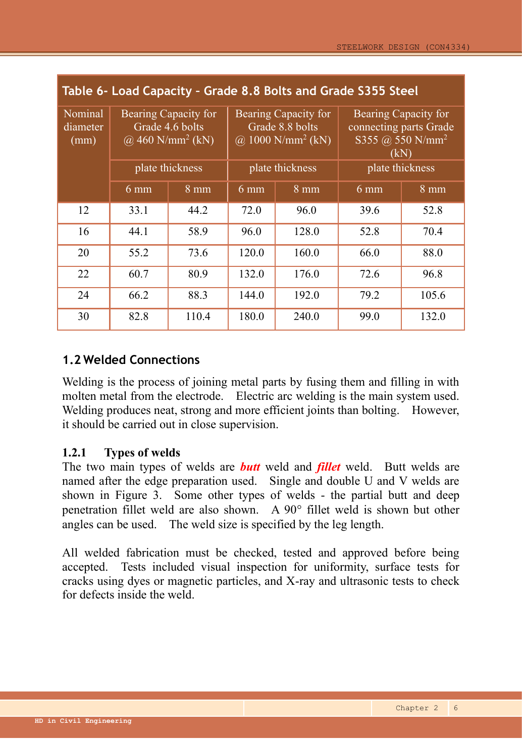
Nominal diameter (); Bearing Capacity (); plate thickness. The left Grade 4.6 group uses bearing stress ; the middle Grade 8.8 group uses ; the right S355 connected-part group uses . In each group the left column has plate thickness and the right column . Displayed source values have truncation/rounding differences. The working below uses unrounded products without forcing them to equal the table entries.
The lower half of the original page begins section 1.2, Welded Connections. Welding joins fused parent metal and molten filler from an electrode, mainly by arc welding. The lecture describes neat, strong and efficient joints requiring close supervision. Section 1.2.1 lists butt and fillet welds as the main types. Butt welds are named by edge preparation; Figure 3 shows single/double U and V preparations, partial butt welds and deep-penetration fillet welds. The illustrated fillet weld angle is ; other angles are possible. Weld size is specified by leg length. Completed work must be inspected, tested and accepted, including visual uniformity, dye or magnetic-particle surface-crack tests, and X-ray or ultrasonic inspection for internal defects.
Animation labBearing and the remaining ligament
Supplement to the original lesson. Enable JavaScript to play, step through calculations and rotate 3D models. The following explanation remains readable offline.
- Force transfers through contact between bolt and connected plate.
- The plate around the hole carries bearing stress. Bolt bearing and plate bearing are separate checks.
- A short ligament can tear out towards the end. The direction of force determines the relevant edge.
- Evaluate every specified bearing and ligament bound for each layer and retain the smallest applicable resistance.
M12: all six bearing cells
Given nominal diameter . Required: six projected-bearing capacities. Select the correct column by bolt/plate material and contacted plate thickness; never use hole diameter here.
Grade 4.6 bolt, plate. Contact area=; resistance=area×bearing stress.
Grade 4.6 bolt, plate. Contact area=; resistance=area×bearing stress.
Grade 8.8 bolt, plate. Contact area=; resistance=area×bearing stress.
Grade 8.8 bolt, plate. Contact area=; resistance=area×bearing stress.
S355 connected plate, , plate. Contact area=; resistance=area×bearing stress.
S355 connected plate, , plate. Contact area=; resistance=area×bearing stress.
Try it yourself. Would doubling end distance double all six M12 table values?
Reveal answer and reasoning
No. These diameter-based values are independent of end distance. A separate end-distance-limited resistance may increase until another limit governs.
Animation labBearing and the remaining ligament
Supplement to the original lesson. Enable JavaScript to play, step through calculations and rotate 3D models. The following explanation remains readable offline.
- Force transfers through contact between bolt and connected plate.
- The plate around the hole carries bearing stress. Bolt bearing and plate bearing are separate checks.
- A short ligament can tear out towards the end. The direction of force determines the relevant edge.
- Evaluate every specified bearing and ligament bound for each layer and retain the smallest applicable resistance.
M16: all six bearing cells
Given nominal diameter . Required: six projected-bearing capacities. Select the correct column by bolt/plate material and contacted plate thickness; never use hole diameter here.
Grade 4.6 bolt, plate. Contact area=; resistance=area×bearing stress.
Grade 4.6 bolt, plate. Contact area=; resistance=area×bearing stress.
Grade 8.8 bolt, plate. Contact area=; resistance=area×bearing stress.
Grade 8.8 bolt, plate. Contact area=; resistance=area×bearing stress.
S355 connected plate, , plate. Contact area=; resistance=area×bearing stress.
S355 connected plate, , plate. Contact area=; resistance=area×bearing stress.
Try it yourself. Would doubling end distance double all six M16 table values?
Reveal answer and reasoning
No. These diameter-based values are independent of end distance. A separate end-distance-limited resistance may increase until another limit governs.
Animation labBearing and the remaining ligament
Supplement to the original lesson. Enable JavaScript to play, step through calculations and rotate 3D models. The following explanation remains readable offline.
- Force transfers through contact between bolt and connected plate.
- The plate around the hole carries bearing stress. Bolt bearing and plate bearing are separate checks.
- A short ligament can tear out towards the end. The direction of force determines the relevant edge.
- Evaluate every specified bearing and ligament bound for each layer and retain the smallest applicable resistance.
M20: all six bearing cells
Given nominal diameter . Required: six projected-bearing capacities. Select the correct column by bolt/plate material and contacted plate thickness; never use hole diameter here.
Grade 4.6 bolt, plate. Contact area=; resistance=area×bearing stress.
Grade 4.6 bolt, plate. Contact area=; resistance=area×bearing stress.
Grade 8.8 bolt, plate. Contact area=; resistance=area×bearing stress.
Grade 8.8 bolt, plate. Contact area=; resistance=area×bearing stress.
S355 connected plate, , plate. Contact area=; resistance=area×bearing stress.
S355 connected plate, , plate. Contact area=; resistance=area×bearing stress.
Try it yourself. Would doubling end distance double all six M20 table values?
Reveal answer and reasoning
No. These diameter-based values are independent of end distance. A separate end-distance-limited resistance may increase until another limit governs.
Animation labBearing and the remaining ligament
Supplement to the original lesson. Enable JavaScript to play, step through calculations and rotate 3D models. The following explanation remains readable offline.
- Force transfers through contact between bolt and connected plate.
- The plate around the hole carries bearing stress. Bolt bearing and plate bearing are separate checks.
- A short ligament can tear out towards the end. The direction of force determines the relevant edge.
- Evaluate every specified bearing and ligament bound for each layer and retain the smallest applicable resistance.
M22: all six bearing cells
Given nominal diameter . Required: six projected-bearing capacities. Select the correct column by bolt/plate material and contacted plate thickness; never use hole diameter here.
Grade 4.6 bolt, plate. Contact area=; resistance=area×bearing stress.
Grade 4.6 bolt, plate. Contact area=; resistance=area×bearing stress.
Grade 8.8 bolt, plate. Contact area=; resistance=area×bearing stress.
Grade 8.8 bolt, plate. Contact area=; resistance=area×bearing stress.
S355 connected plate, , plate. Contact area=; resistance=area×bearing stress.
S355 connected plate, , plate. Contact area=; resistance=area×bearing stress.
Try it yourself. Would doubling end distance double all six M22 table values?
Reveal answer and reasoning
No. These diameter-based values are independent of end distance. A separate end-distance-limited resistance may increase until another limit governs.
Animation labBearing and the remaining ligament
Supplement to the original lesson. Enable JavaScript to play, step through calculations and rotate 3D models. The following explanation remains readable offline.
- Force transfers through contact between bolt and connected plate.
- The plate around the hole carries bearing stress. Bolt bearing and plate bearing are separate checks.
- A short ligament can tear out towards the end. The direction of force determines the relevant edge.
- Evaluate every specified bearing and ligament bound for each layer and retain the smallest applicable resistance.
M24: all six bearing cells
Given nominal diameter . Required: six projected-bearing capacities. Select the correct column by bolt/plate material and contacted plate thickness; never use hole diameter here.
Grade 4.6 bolt, plate. Contact area=; resistance=area×bearing stress.
Grade 4.6 bolt, plate. Contact area=; resistance=area×bearing stress.
Grade 8.8 bolt, plate. Contact area=; resistance=area×bearing stress.
Grade 8.8 bolt, plate. Contact area=; resistance=area×bearing stress.
S355 connected plate, , plate. Contact area=; resistance=area×bearing stress.
S355 connected plate, , plate. Contact area=; resistance=area×bearing stress.
Try it yourself. Would doubling end distance double all six M24 table values?
Reveal answer and reasoning
No. These diameter-based values are independent of end distance. A separate end-distance-limited resistance may increase until another limit governs.
Animation labBearing and the remaining ligament
Supplement to the original lesson. Enable JavaScript to play, step through calculations and rotate 3D models. The following explanation remains readable offline.
- Force transfers through contact between bolt and connected plate.
- The plate around the hole carries bearing stress. Bolt bearing and plate bearing are separate checks.
- A short ligament can tear out towards the end. The direction of force determines the relevant edge.
- Evaluate every specified bearing and ligament bound for each layer and retain the smallest applicable resistance.
M30: all six bearing cells
Given nominal diameter . Required: six projected-bearing capacities. Select the correct column by bolt/plate material and contacted plate thickness; never use hole diameter here.
Grade 4.6 bolt, plate. Contact area=; resistance=area×bearing stress.
Grade 4.6 bolt, plate. Contact area=; resistance=area×bearing stress.
Grade 8.8 bolt, plate. Contact area=; resistance=area×bearing stress.
Grade 8.8 bolt, plate. Contact area=; resistance=area×bearing stress.
S355 connected plate, , plate. Contact area=; resistance=area×bearing stress.
S355 connected plate, , plate. Contact area=; resistance=area×bearing stress.
Try it yourself. Would doubling end distance double all six M30 table values?
Reveal answer and reasoning
No. These diameter-based values are independent of end distance. A separate end-distance-limited resistance may increase until another limit governs.
Animation labBearing and the remaining ligament
Supplement to the original lesson. Enable JavaScript to play, step through calculations and rotate 3D models. The following explanation remains readable offline.
- Force transfers through contact between bolt and connected plate.
- The plate around the hole carries bearing stress. Bolt bearing and plate bearing are separate checks.
- A short ligament can tear out towards the end. The direction of force determines the relevant edge.
- Evaluate every specified bearing and ligament bound for each layer and retain the smallest applicable resistance.
Rebuild every cell of the lecture fillet-weld table
Source: Chapter 2 p.31, Tables 10 and 11. fillet weld has throat . A weld of length has throat area , so resistance per millimetre is . Match steel grade and electrode class together: S275/Class 35 uses ; S355/Class 42 or 50 uses ; S460/Class 50 uses . Increasing electrode class alone does not turn the S275-row strength into .
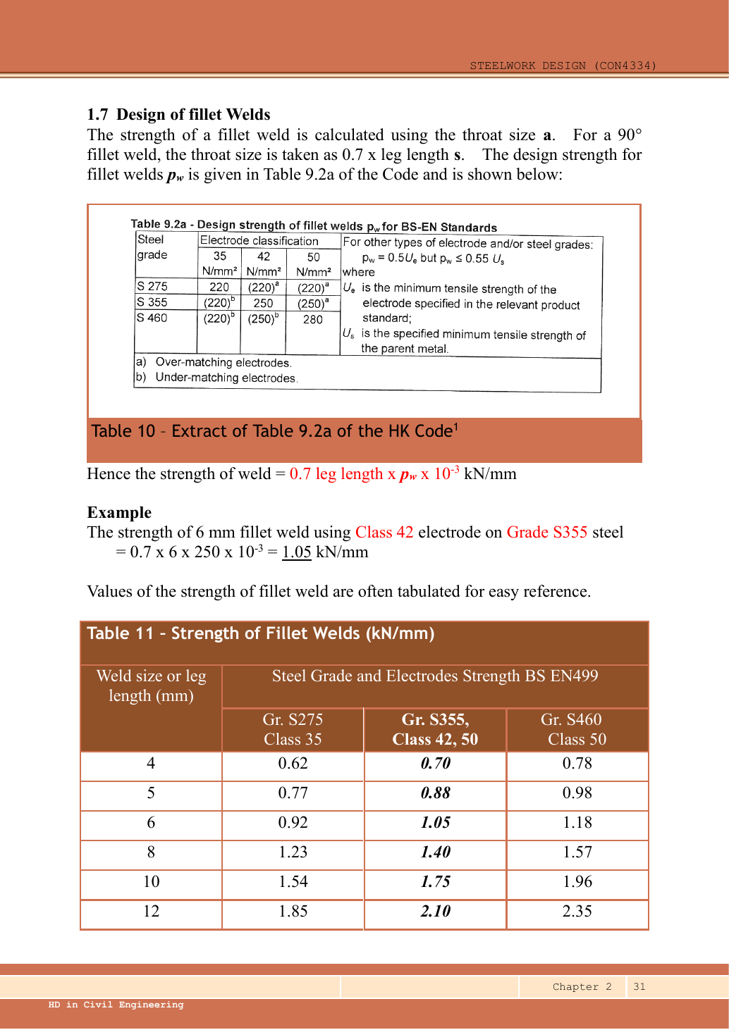
Section 1.7, Design of Fillet Welds: calculate strength using throat ; for , , is leg length. Table 10 extracts Hong Kong code Table 9.2a; headings identify steel grade and electrode classification, with all strengths in . Under Classes 35/42/50, S275 gives respectively ; S355 ; S460 . Superscript a denotes over-matching and b under-matching electrode strength; source parentheses/superscripts remain visible in the image. For other electrode/steel combinations, use , but ; is the electrode's minimum tensile strength specified by the product standard; is the parent metal's specified minimum tensile strength.
The diagram gives resistance per unit length as . Example: S355 with Class 42 and weld leg ,. Table 11 labels Weld size or leg length (); its three columns pair S275/Class 35, S355/Class 42 or 50, and S460/Class 50. The BS EN499 heading is retained. Table values are resistance per millimetre () for convenient lookup, not the force in the whole weld.
Animation labFrom fillet leg to effective throat
Supplement to the original lesson. Enable JavaScript to play, step through calculations and rotate 3D models. The following explanation remains readable offline.
- An equal-leg fillet between perpendicular plates has an approximately right-triangular section.
- For this geometry, throat . It is shorter than the leg.
- Effective resisting area = . With here, capacity per length is .
- Use the course end allowances, minimum size and length rules; increasing the geometric length alone does not resolve every detailing check.
fillet: all three material cells
Given leg . Calculated throat . Required: strength per millimetre for each of the three printed material columns.
S275 / Class 35: lookup . Multiply throat area per unit run by .
S355 / Class 42 or 50: lookup . Multiply throat area per unit run by .
S460 / Class 50: lookup . Multiply throat area per unit run by .
Choose effective weld length from demand/q and check physical-length deductions, minimum length, minimum/maximum size, lap and returns. A table row is not a complete weld detail.
Try it yourself. What force corresponds to effective S355/Class 42 weld of leg ?
Reveal answer and reasoning
, subject to the separate detailing and parent-metal checks.
Animation labFrom fillet leg to effective throat
Supplement to the original lesson. Enable JavaScript to play, step through calculations and rotate 3D models. The following explanation remains readable offline.
- An equal-leg fillet between perpendicular plates has an approximately right-triangular section.
- For this geometry, throat . It is shorter than the leg.
- Effective resisting area = . With here, capacity per length is .
- Use the course end allowances, minimum size and length rules; increasing the geometric length alone does not resolve every detailing check.
Animation labFrom fillet leg to effective throat
Supplement to the original lesson. Enable JavaScript to play, step through calculations and rotate 3D models. The following explanation remains readable offline.
- An equal-leg fillet between perpendicular plates has an approximately right-triangular section.
- For this geometry, throat . It is shorter than the leg.
- Effective resisting area = . With here, capacity per length is .
- Use the course end allowances, minimum size and length rules; increasing the geometric length alone does not resolve every detailing check.
fillet: all three material cells
Given leg . Calculated throat . Required: strength per millimetre for each of the three printed material columns.
S275 / Class 35: lookup . Multiply throat area per unit run by .
S355 / Class 42 or 50: lookup . Multiply throat area per unit run by .
S460 / Class 50: lookup . Multiply throat area per unit run by .
Choose effective weld length from demand/q and check physical-length deductions, minimum length, minimum/maximum size, lap and returns. A table row is not a complete weld detail.
Try it yourself. What force corresponds to effective S355/Class 42 weld of leg ?
Reveal answer and reasoning
, subject to the separate detailing and parent-metal checks.
Animation labFrom fillet leg to effective throat
Supplement to the original lesson. Enable JavaScript to play, step through calculations and rotate 3D models. The following explanation remains readable offline.
- An equal-leg fillet between perpendicular plates has an approximately right-triangular section.
- For this geometry, throat . It is shorter than the leg.
- Effective resisting area = . With here, capacity per length is .
- Use the course end allowances, minimum size and length rules; increasing the geometric length alone does not resolve every detailing check.
Animation labFrom fillet leg to effective throat
Supplement to the original lesson. Enable JavaScript to play, step through calculations and rotate 3D models. The following explanation remains readable offline.
- An equal-leg fillet between perpendicular plates has an approximately right-triangular section.
- For this geometry, throat . It is shorter than the leg.
- Effective resisting area = . With here, capacity per length is .
- Use the course end allowances, minimum size and length rules; increasing the geometric length alone does not resolve every detailing check.
fillet: all three material cells
Given leg . Calculated throat . Required: strength per millimetre for each of the three printed material columns.
S275 / Class 35: lookup . Multiply throat area per unit run by .
S355 / Class 42 or 50: lookup . Multiply throat area per unit run by .
S460 / Class 50: lookup . Multiply throat area per unit run by .
Choose effective weld length from demand/q and check physical-length deductions, minimum length, minimum/maximum size, lap and returns. A table row is not a complete weld detail.
Try it yourself. What force corresponds to effective S355/Class 42 weld of leg ?
Reveal answer and reasoning
, subject to the separate detailing and parent-metal checks.
Animation labFrom fillet leg to effective throat
Supplement to the original lesson. Enable JavaScript to play, step through calculations and rotate 3D models. The following explanation remains readable offline.
- An equal-leg fillet between perpendicular plates has an approximately right-triangular section.
- For this geometry, throat . It is shorter than the leg.
- Effective resisting area = . With here, capacity per length is .
- Use the course end allowances, minimum size and length rules; increasing the geometric length alone does not resolve every detailing check.
Animation labFrom fillet leg to effective throat
Supplement to the original lesson. Enable JavaScript to play, step through calculations and rotate 3D models. The following explanation remains readable offline.
- An equal-leg fillet between perpendicular plates has an approximately right-triangular section.
- For this geometry, throat . It is shorter than the leg.
- Effective resisting area = . With here, capacity per length is .
- Use the course end allowances, minimum size and length rules; increasing the geometric length alone does not resolve every detailing check.
fillet: all three material cells
Given leg . Calculated throat . Required: strength per millimetre for each of the three printed material columns.
S275 / Class 35: lookup . Multiply throat area per unit run by .
S355 / Class 42 or 50: lookup . Multiply throat area per unit run by .
S460 / Class 50: lookup . Multiply throat area per unit run by .
Choose effective weld length from demand/q and check physical-length deductions, minimum length, minimum/maximum size, lap and returns. A table row is not a complete weld detail.
Try it yourself. What force corresponds to effective S355/Class 42 weld of leg ?
Reveal answer and reasoning
, subject to the separate detailing and parent-metal checks.
Animation labFrom fillet leg to effective throat
Supplement to the original lesson. Enable JavaScript to play, step through calculations and rotate 3D models. The following explanation remains readable offline.
- An equal-leg fillet between perpendicular plates has an approximately right-triangular section.
- For this geometry, throat . It is shorter than the leg.
- Effective resisting area = . With here, capacity per length is .
- Use the course end allowances, minimum size and length rules; increasing the geometric length alone does not resolve every detailing check.
Animation labFrom fillet leg to effective throat
Supplement to the original lesson. Enable JavaScript to play, step through calculations and rotate 3D models. The following explanation remains readable offline.
- An equal-leg fillet between perpendicular plates has an approximately right-triangular section.
- For this geometry, throat . It is shorter than the leg.
- Effective resisting area = . With here, capacity per length is .
- Use the course end allowances, minimum size and length rules; increasing the geometric length alone does not resolve every detailing check.
fillet: all three material cells
Given leg . Calculated throat . Required: strength per millimetre for each of the three printed material columns.
S275 / Class 35: lookup . Multiply throat area per unit run by .
S355 / Class 42 or 50: lookup . Multiply throat area per unit run by .
S460 / Class 50: lookup . Multiply throat area per unit run by .
Choose effective weld length from demand/q and check physical-length deductions, minimum length, minimum/maximum size, lap and returns. A table row is not a complete weld detail.
Try it yourself. What force corresponds to effective S355/Class 42 weld of leg ?
Reveal answer and reasoning
, subject to the separate detailing and parent-metal checks.
Animation labFrom fillet leg to effective throat
Supplement to the original lesson. Enable JavaScript to play, step through calculations and rotate 3D models. The following explanation remains readable offline.
- An equal-leg fillet between perpendicular plates has an approximately right-triangular section.
- For this geometry, throat . It is shorter than the leg.
- Effective resisting area = . With here, capacity per length is .
- Use the course end allowances, minimum size and length rules; increasing the geometric length alone does not resolve every detailing check.
Animation labFrom fillet leg to effective throat
Supplement to the original lesson. Enable JavaScript to play, step through calculations and rotate 3D models. The following explanation remains readable offline.
- An equal-leg fillet between perpendicular plates has an approximately right-triangular section.
- For this geometry, throat . It is shorter than the leg.
- Effective resisting area = . With here, capacity per length is .
- Use the course end allowances, minimum size and length rules; increasing the geometric length alone does not resolve every detailing check.
fillet: all three material cells
Given leg . Calculated throat . Required: strength per millimetre for each of the three printed material columns.
S275 / Class 35: lookup . Multiply throat area per unit run by .
S355 / Class 42 or 50: lookup . Multiply throat area per unit run by .
S460 / Class 50: lookup . Multiply throat area per unit run by .
Choose effective weld length from demand/q and check physical-length deductions, minimum length, minimum/maximum size, lap and returns. A table row is not a complete weld detail.
Try it yourself. What force corresponds to effective S355/Class 42 weld of leg ?
Reveal answer and reasoning
, subject to the separate detailing and parent-metal checks.
Animation labFrom fillet leg to effective throat
Supplement to the original lesson. Enable JavaScript to play, step through calculations and rotate 3D models. The following explanation remains readable offline.
- An equal-leg fillet between perpendicular plates has an approximately right-triangular section.
- For this geometry, throat . It is shorter than the leg.
- Effective resisting area = . With here, capacity per length is .
- Use the course end allowances, minimum size and length rules; increasing the geometric length alone does not resolve every detailing check.
Animation labFrom fillet leg to effective throat
Supplement to the original lesson. Enable JavaScript to play, step through calculations and rotate 3D models. The following explanation remains readable offline.
- An equal-leg fillet between perpendicular plates has an approximately right-triangular section.
- For this geometry, throat . It is shorter than the leg.
- Effective resisting area = . With here, capacity per length is .
- Use the course end allowances, minimum size and length rules; increasing the geometric length alone does not resolve every detailing check.