Worked examples

Column example 5: axial load plus biaxial end moments

Open “Animation lab” beside a teaching step for a visual explanation or a walkthrough of its original expressions. Models are illustrative; source answers remain unchanged.

← Read this lecture example beside its chapter concepts

Chinese–English terminology

Need a simpler picture? Open “Simple explanation” beside a difficult step. These optional notes do not replace the full solution.

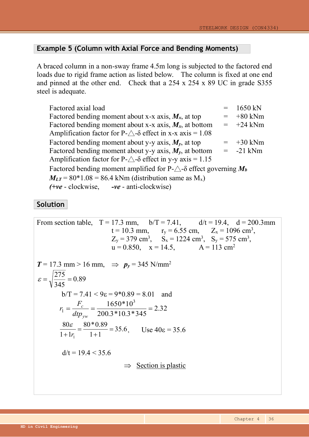
Check a $254 \times 254 \times 89$ UC S355 column in a braced non-sway frame, $4.5 m$ long, fixed at one end and pinned at the other. Design compression is $1,650 kN$ . First-order factored end moments are $M_{x}$ (top/bottom)= $+ 80$ / $+ 24 kN \cdot m$ and Mᵧ(top/bottom)= $+ 30$ / $- 21 kN \cdot m$ . Amplification factors are $1.08$ about $x$ and $1.15$ about $y$ . The given amplified Mᴸᵀ=86.4 kNm has the same distribution as $M_{x}$ .

Original source: LectureNotes/Ch 4_Column.pdf — p. 36, p. 37, p. 38. Values tagged given are in the question or diagram; lookup values come from a named table; calculated values follow from the working; assumptions are stated explicitly.

Ch 4 p.36 supplies a load table, not a structural sketch. Clockwise moments are positive and anticlockwise moments negative. Top/bottom identify member ends; factored loads already include partial load factors; the amplification factor increases the moment.

4.5 m

length and the fixed/pinned-end wording establish the model. The source table writes the amplification effect as

P - Δ - δ

; its original expression for the already amplified moment is

M_{LT} = 80 \times 1.08 = 86.4 kN \cdot m

, with the same distribution as

M_{x}

. The main explanation also uses

M^{LT}

for that same given moment, not a separate unamplified input. The source load table and sign convention are retained; no new dimensions are inferred. End moments and section properties are typeset step by step below.Open full-size image

Read the diagram and collect the data

Input	Meaning/value source
End moments	Given applied-arrow convention: $+ 80$ / $+ 24$ about $x$ ; $+ 30$ / $- 21$ about $y$ . Convert to the Table 8.9 internal-diagram ratio.
Amplification	Given $1.08$ and $1.15$ ; Mᴸᵀ86.4 already includes amplification.
Section row	Data File p.11, $254 \times 254 \times 89$ UC: $T = 17.3$ , $t = 10.3$ , $d = 200.3 mm$ ; $\frac{b}{T} = 7.41$ , $\frac{d}{t} = 19.4$ ; $r_{x} = 11.2 cm$ , $r_{y} = 6.55 cm$ ; $A = 113 {cm}^{2}$ ; $Z_{x} = 1,096$ , $Z_{y} = 379$ , $S_{x} = 1,224$ , $S_{y} = 575 {cm}^{3}$ ; $u = 0.850$ , $x = 14.5$ .
Restraint/curve choices	Table 8.6 recommended fixed/pinned K0.85; rolled H $\leq 40 mm$ uses b about $x$ ,c about $y$ .

Before calculating: recognition and strategy

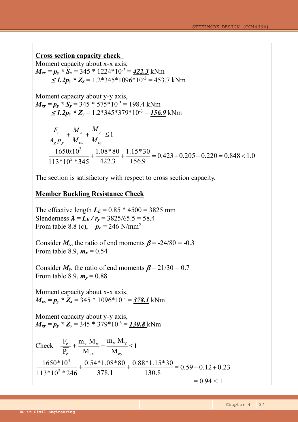
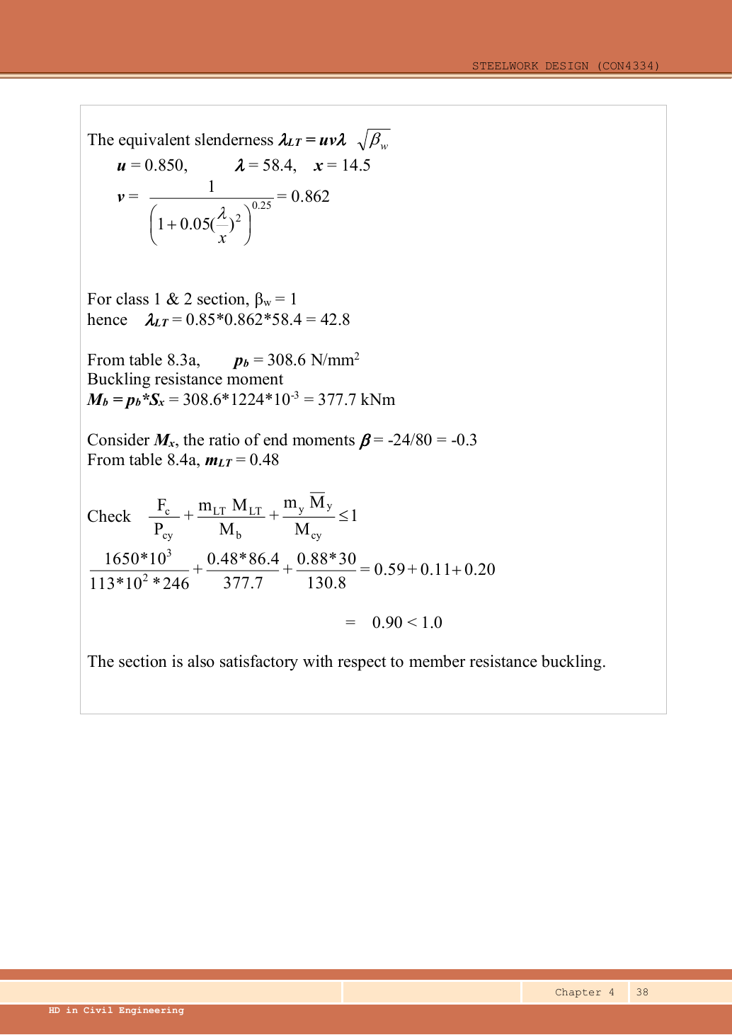
This is continuous-frame end-moment design, so use the full $u - v$ LTB procedure and moment factors from the separate flexural/LTB tables. Check three things: local section interaction, flexural member interaction, and axial/LTB interaction. The section moment denominator is capped plastic resistance, whereas the member denominators are elastic pᵧZ. The source’s LTB minor-axis term uses first-order Mᵧ; its flexural term uses amplified Mᵧ.

1. Strength, combined-stress classification and moments

T = 17.3 mm

lies within

16 < T \leq 40

, so

p_{y} = 345 \frac{N}{{mm}^{2}}

ε = \sqrt{\frac{275}{345}} = 0.892805

Class 1 flange limit

9 ε = 8.03525

;

\frac{b}{T} = 7.41 < 8.03525

. Web compression ratio:

r_{1} = \frac{F_{c}}{d t p_{y}}

= \frac{1,650,000}{200.3 \times 10.3 \times 345} \approx 2.318

Under the supplied classification rule,

r_{1}

is limited to

1

. Class 1 web limit:

\frac{80 ε}{1 + r_{1}} = \frac{80 \times 0.892805}{2} = 35.7122

\frac{d}{t} = 19.4 < 35.7122

, so the web is Class 1 and the overall section is Class 1.

M_{x, amp} = 1.08 \times 80 = 86.4 kN \cdot m

M_{y, amp} = 1.15 \times 30 = 34.5 kN \cdot m; M_{y, first} = 30 kN \cdot m

Given

M_{LT} = 86.4 kN \cdot m

; do not amplify it again.

The raw $r_{1}$ exceeds $1$ because the axial load is divided by the web’s $d t$ area, not total section area. The course classification parameter is bounded; this does not mean gross-area compression exceeds capacity.

Animation labWhy thin elements buckle locally2 concepts · 1 source expressions

Supplement to the original lesson. Enable JavaScript to play, step through calculations and rotate 3D models. The following explanation remains readable offline.

The flange outstand and web have different widths, thicknesses and edge support conditions.
A thinner plate can wrinkle locally before the complete member loses stability.
Class 1 allows plastic rotation; Class 2 reaches plastic resistance; Class 3 reaches elastic resistance; Class 4 requires effective properties.
Check every relevant compression element with the supplied limits and stress distribution. The deformation shown is qualitative.

2. Cross-section interaction

Simple explanation: The column needs more than one pass

A slice can be strong while the whole member still buckles.

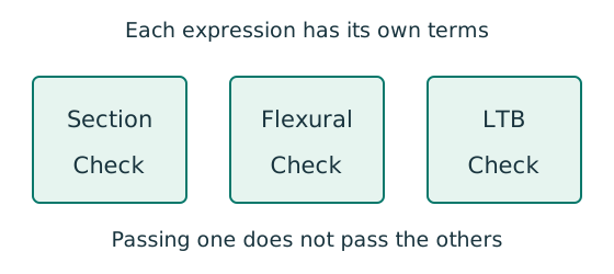
Check cross-section compression plus bending.
Then check the separate member-buckling expressions.
Keep each moment, factor and resistance in its specified expression.

Remember: The three checks do not share interchangeable denominators.

Related concept and full method

A_{g} p_{y} = \frac{113 \times 100 \times 345}{1,000} = 3,898.5 kN

Major axis:

p_{y} S_{x} = \frac{345 \times 1,224}{1,000} = 422.28 kN \cdot m

Upper cap:

1.2 p_{y} Z_{x} = \frac{1.2 \times 345 \times 1,096}{1,000} = 453.744 kN \cdot m

M_{cx} = 422.28 kN \cdot m

Minor axis:

p_{y} S_{y} = \frac{345 \times 575}{1,000} = 198.375 kN \cdot m

Upper cap:

1.2 p_{y} Z_{y} = \frac{1.2 \times 345 \times 379}{1,000} = 156.906 kN \cdot m

M_{cy} = 156.906 kN \cdot m

Utilisation:

\frac{1,650}{3,898.5} + \frac{86.4}{422.28} + \frac{34.5}{156.906}

= 0.847720 < 1

Section passes.

Both maximum moment magnitudes occur at the top in the given load schedule, so they coexist with the stated compression there. The minor-axis ceiling is the governing branch for $M_{cy}$ .

Animation labA strong slice can belong to an unstable member2 concepts · 1 source expressions

Supplement to the original lesson. Enable JavaScript to play, step through calculations and rotate 3D models. The following explanation remains readable offline.

Combine axial compression and the two bending demands using the specified section resistances.
The whole member adds effective-length and buckling-curve effects.
This uses its own moment factor and bending resistance; it is not a copy of the section check.
Elastic, plastic and buckling resistances are not interchangeable. Read the three original expressions and their first-order/amplified moments.

3. Effective length and both axial buckling resistances

L_{Ex} = L_{Ey} = 0.85 \times 4,500 = 3,825 mm

r_{x} = 112 mm; r_{y} = 65.5 mm

λ_{x} = \frac{3,825}{112} = 34.151786

λ_{y} = \frac{3,825}{65.5} = 58.396947

Select curve b for $x$ and c for $y$ ; both use pᵧ345. The source shows only the controlling $y$ result; the $x$ lookup below completes the omitted comparison.

Curve b,

x

axis:

30

row gives

325

，

35

row gives

318 \frac{N}{{mm}^{2}}

. Interpolation fraction:

\frac{34.151786 - 30}{35 - 30} = 0.830357

p_{c} = 325 + 0.830357 \times (318 - 325) = 319.187500 \frac{N}{{mm}^{2}}

Curve c,

y

axis:

58

row gives

247

，

60

row gives

241 \frac{N}{{mm}^{2}}

. Interpolation fraction:

\frac{58.396947 - 58}{60 - 58} = 0.198473

p_{c} = 247 + 0.198473 \times (241 - 247) = 245.809160 \frac{N}{{mm}^{2}}

P_{cx} = \frac{113 \times 319.187500}{10} = 3606.818750 kN

P_{cy} = \frac{113 \times 245.809160}{10} = 2777.643511 kN

P_{c} = P_{cy} = 2777.643511 kN

Animation labEffective length and buckling axes3 concepts · 2 source expressions

Supplement to the original lesson. Enable JavaScript to play, step through calculations and rotate 3D models. The following explanation remains readable offline.

A column can bow sideways before its section reaches the crushing resistance.
Each axis has its own radius of gyration and restraint spacing.
$λ = \frac{L _{E}}{r}$ , with compatible length units. A tie affects only the directions it actually restrains.
Select each buckling curve and compressive strength before forming Pc. The governing axis is determined by resistance, not slenderness alone.

4. Read the two flexural factors and the LTB factor

Simple explanation: Similar-looking moment factors come from different tables

Two recipes can use the same ingredients but different amounts.

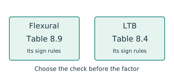
Identify flexural buckling or lateral-torsional buckling first.
Read the actual moment diagram, including any change of sign.
Use that check’s table and its own sign and minimum-factor rules.

Remember: Table 8.9 flexural factors are not Table 8.4 LTB factors.

Related concept and full method

The question defines signs for applied clockwise/anticlockwise end moments. The internal end-moment diagram reverses the bottom-end sign relative to that schedule. Thus the same positive applied signs about $x$ create a reversing BMD, while the opposite applied signs about $y$ create a same-side BMD.

β_{x} = \frac{- 24}{80} = - 0.3

Table 8.9:

m_{x} = 0.54

β_{y} = \frac{- (- 21)}{30} = + 0.7

Table 8.9:

m_{y} = 0.88

M_{LT}

and

x

axis has the same moment-diagram shape;

β = - 0.3

. Table 8.4a:

m_{LT} = 0.48

Do not read $0.48$ as $m_{x}$ : that belongs to the different LTB table. Uniform amplification about an axis multiplies both ends equally and leaves the end-moment ratio unchanged.

Animation labRead the moment shape within one segment3 concepts · 1 source expressions

Supplement to the original lesson. Enable JavaScript to play, step through calculations and rotate 3D models. The following explanation remains readable offline.

Moment ordinates must belong to the same effective unbraced segment.
Same-side and reverse-curvature diagrams have different signed end ratios.
The markers show ¼, ½ and ¾ of this segment, not of the entire beam.
LTB and column flexural factors are different. Preserve their individual bounds and coefficient sets.

5. Flexural member interaction with elastic denominators

M_{ex} = p_{y} Z_{x} = \frac{345 \times 1,096}{1,000} = 378.12 kN \cdot m

M_{ey} = p_{y} Z_{y} = \frac{345 \times 379}{1,000} = 130.755 kN \cdot m

U_{flex} = \frac{1,650}{2777.643511} + \frac{0.54 \times 86.4}{378.12} + \frac{0.88 \times 34.5}{130.755}

= 0.594029 + 0.123389 + 0.232190

= 0.949608 < 1

Passes.

Animation labA strong slice can belong to an unstable member2 concepts · 1 source expressions

Supplement to the original lesson. Enable JavaScript to play, step through calculations and rotate 3D models. The following explanation remains readable offline.

Combine axial compression and the two bending demands using the specified section resistances.
The whole member adds effective-length and buckling-curve effects.
This uses its own moment factor and bending resistance; it is not a copy of the section check.
Elastic, plastic and buckling resistances are not interchangeable. Read the three original expressions and their first-order/amplified moments.

6. Axial/LTB interaction

Simple explanation: A beam can escape sideways

The compressed flange can move sideways while the section twists.

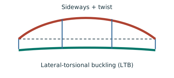
Divide the beam at effective lateral restraints.
Use each segment’s effective length to obtain its buckling resistance.
Compare that resistance with the segment’s equivalent moment demand.

Remember: A section bending check alone does not check lateral-torsional buckling.

Related concept and full method

λ = 58.396947

; section torsional index

x = 14.5

v = {[1 + 0.05 {(\frac{58.396947}{14.5})}^{2}]}^{- 0.25} = 0.862028

β_{w} = 1; λ_{LT} = 0.850 \times 0.862028 \times 58.396947 = 42.788808

Table 8.3a，

p_{y} = 345

column:

40

row gives

317

，

45

row gives

302 \frac{N}{{mm}^{2}}

. Interpolation fraction:

\frac{42.788808 - 40}{45 - 40} = 0.557762

p_{b} = 317 + 0.557762 \times (302 - 317) = 308.633576 \frac{N}{{mm}^{2}}

M_{b} = \frac{308.633576 \times 1,224}{1,000} = 377.767497 kN \cdot m

U_{LT} = \frac{1,650}{2777.643511} + \frac{0.48 \times 86.4}{377.767497} + \frac{0.88 \times 30}{130.755}

= 0.594029 + 0.109782 + 0.201904

= 0.905715 < 1

Passes.

The $30 kN \cdot m$ in the last term is intentional: source Eq.8.81 has barred, first-order Mᵧ. The $86.4 kN \cdot m$ Mᴸᵀ is already amplified. All three interactions pass; flexural member interaction is closest to $1$ .

Animation labA strong slice can belong to an unstable member5 concepts · 1 source expressions

Supplement to the original lesson. Enable JavaScript to play, step through calculations and rotate 3D models. The following explanation remains readable offline.

Combine axial compression and the two bending demands using the specified section resistances.
The whole member adds effective-length and buckling-curve effects.
This uses its own moment factor and bending resistance; it is not a copy of the section check.
Elastic, plastic and buckling resistances are not interchangeable. Read the three original expressions and their first-order/amplified moments.

Compact exam answer

S355 $254 \times 254 \times 89$ UC: $p_{y} = 345$ , Class 1. Section utilisation $0.84772$ . $L^{E} = 3,825 mm$ ; $λ_{x} = 34.1518$ , $λ_{y} = 58.3969$ ; curves b/c give $p_{cx} = 319.1875$ , $p_{cy} = 245.8092 \frac{N}{{mm}^{2}}$ . $P_{c} = P_{cy} = 2,777.6435 kN$ . $m_{x} = 0.54$ , $m_{y} = 0.88$ ; elastic resistance $378.12$ ／ $130.755 kN \cdot m$ ; flexural-buckling utilisation $0.94961$ . $v = 0.862028$ , $λ^{LT} = 42.7888$ , $p_{b} = 308.6336$ , $M_{b} = 377.7675 kN \cdot m$ , $m^{LT} = 0.48$ ; axial force/LTB utilisation $0.90571$ . All pass.

Mistakes to avoid

Use $345$ , not $355$ , for the $17.3 mm$ flange.
Apply the 1.2pᵧZ ceiling on the minor axis.
Do not use capped plastic capacities in the member interaction.
Distinguish applied end signs from internal moment-diagram signs.
Keep first-order Mᵧ in the source Eq.8.81 term.

Procedure for an unfamiliar variant

Identify axial load, any moments, actual length and restraints in each axis.
Choose/read a section and confirm strength from the actual thickness.
Check the appropriate flange and web local-slenderness limits.
Find $λ_{x}$ and $λ_{y}$ separately; select each axis curve and interpolate $p_{c}$ .
Calculate both axial resistances and identify the governing axis.
If moments exist, complete section, flexural and axial/LTB interactions using their own capacities and moment definitions.

Independent self-check

Try it yourself. Invented variant: only the imposed major-axis end moments in the given factored schedule are replaced by $+ 88$ / $+ 26.4 kN \cdot m$ ; treat these as a $10 %$ increase of the stated total first-order $x$ moments, with axial load and $y$ moments unchanged. How do the checks change?

Reveal answer and reasoning

$x$ -axis end-moment ratio remains $- 0.3$ , so $m_{x} = 0.54$ , $m^{LT} = 0.48$ are unchanged. $M_{x, amp} = M^{LT} = 1.08 \times 88 = 95.04 kN \cdot m$ . Section utilisation increases by $\frac{8.64}{422.28} \approx 0.02046$ to $0.86818$ . Flexural-buckling utilisation increases by $\frac{0.54 \times 8.64}{378.12} \approx 0.01234$ to $0.96195$ . LTB utilisation increases by $\frac{0.48 \times 8.64}{377.7675} \approx 0.01098$ to $0.91669$ . All still pass, with resistance properties unchanged.

Animation labA strong slice can belong to an unstable member3 concepts · 3 source expressions

Supplement to the original lesson. Enable JavaScript to play, step through calculations and rotate 3D models. The following explanation remains readable offline.

Combine axial compression and the two bending demands using the specified section resistances.
The whole member adds effective-length and buckling-curve effects.
This uses its own moment factor and bending resistance; it is not a copy of the section check.
Elastic, plastic and buckling resistances are not interchangeable. Read the three original expressions and their first-order/amplified moments.